Data Structures LECTURE 15 Shortest paths algorithms Properties

Data Structures – LECTURE 15 Shortest paths algorithms • Properties of shortest paths • Bellman-Ford algorithm • Dijsktra’s algorithm Chapter 24 in the textbook (pp 580– 599). Data Structures, Spring 2006 © L. Joskowicz 1

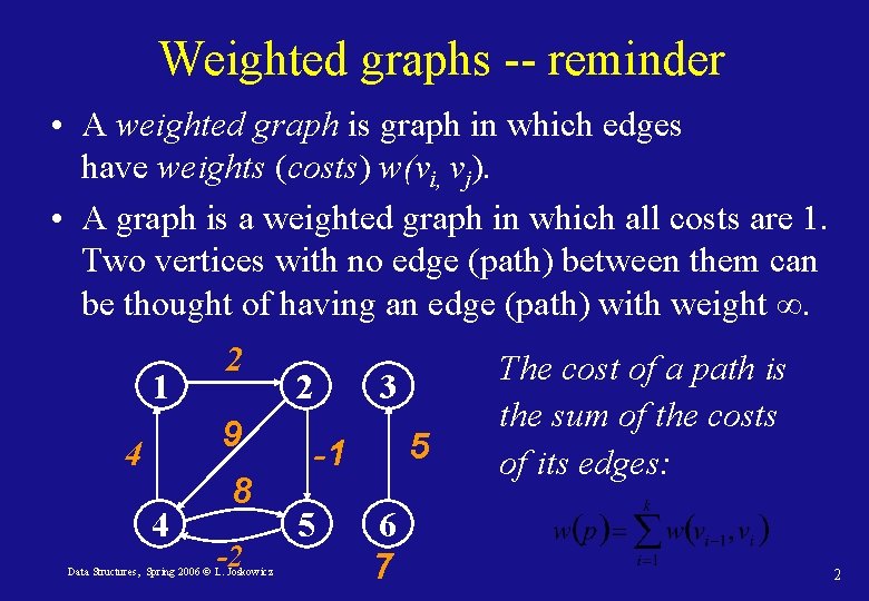
Weighted graphs -- reminder • A weighted graph is graph in which edges have weights (costs) w(vi, vj). • A graph is a weighted graph in which all costs are 1. Two vertices with no edge (path) between them can be thought of having an edge (path) with weight ∞. 1 2 9 4 4 8 -2 Data Structures, Spring 2006 © L. Joskowicz 2 3 5 -1 5 6 7 The cost of a path is the sum of the costs of its edges: 2

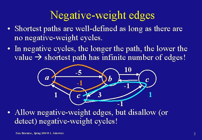
Negative-weight edges • Shortest paths are well-defined as long as there are no negative-weight cycles. • In negative cycles, the longer the path, the lower the value shortest path has infinite number of edges! 10 -5 -1 a 1 c b -1 c 1 3 -1 • Allow negative-weight edges, but disallow (or detect) negative-weight cycles! Data Structures, Spring 2006 © L. Joskowicz 3

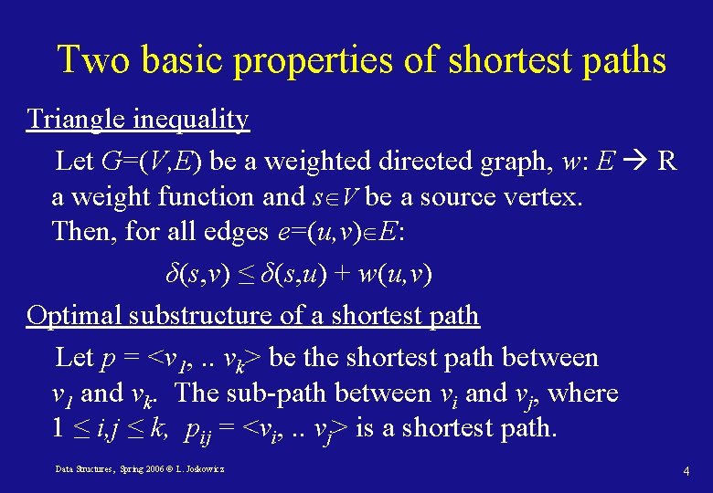
Two basic properties of shortest paths Triangle inequality Let G=(V, E) be a weighted directed graph, w: E R a weight function and s V be a source vertex. Then, for all edges e=(u, v) E: δ(s, v) ≤ δ(s, u) + w(u, v) Optimal substructure of a shortest path Let p = <v 1, . . vk> be the shortest path between v 1 and vk. The sub-path between vi and vj, where 1 ≤ i, j ≤ k, pij = <vi, . . vj> is a shortest path. Data Structures, Spring 2006 © L. Joskowicz 4

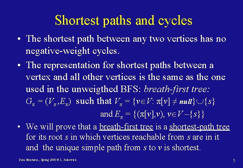
Shortest paths and cycles • The shortest path between any two vertices has no negative-weight cycles. • The representation for shortest paths between a vertex and all other vertices is the same as the one used in the unweigthed BFS: breath-first tree: Gπ = (Vπ , Eπ) such that Vπ = {v V: π[v] ≠ null} {s} and Eπ = {(π[v], v), v V –{s}} • We will prove that a breath-first tree is a shortest-path tree for its root s in which vertices reachable from s are in it and the unique simple path from s to v is shortest. Data Structures, Spring 2006 © L. Joskowicz 5

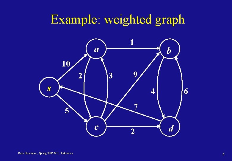
Example: weighted graph 1 a b 10 2 3 9 s 4 7 5 c Data Structures, Spring 2006 © L. Joskowicz 6 2 d 6

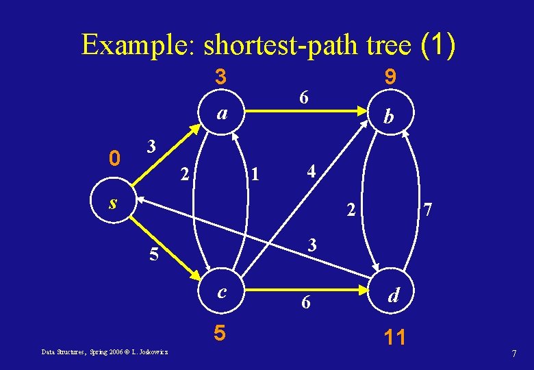
Example: shortest-path tree (1) 3 6 a 0 9 b 3 2 1 4 s 2 3 5 c 5 Data Structures, Spring 2006 © L. Joskowicz 7 6 d 11 7

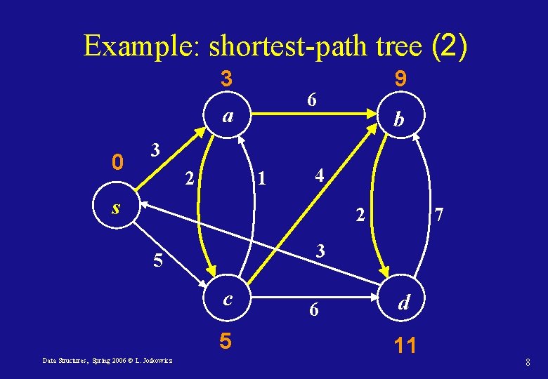
Example: shortest-path tree (2) 3 6 a 0 9 b 3 2 1 4 s 2 3 5 c 5 Data Structures, Spring 2006 © L. Joskowicz 7 6 d 11 8

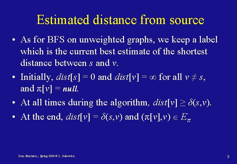
Estimated distance from source • As for BFS on unweighted graphs, we keep a label which is the current best estimate of the shortest distance between s and v. • Initially, dist[s] = 0 and dist[v] = ∞ for all v ≠ s, and π[v] = null. • At all times during the algorithm, dist[v] ≥ δ(s, v). • At the end, dist[v] = δ(s, v) and (π[v], v) Eπ Data Structures, Spring 2006 © L. Joskowicz 9

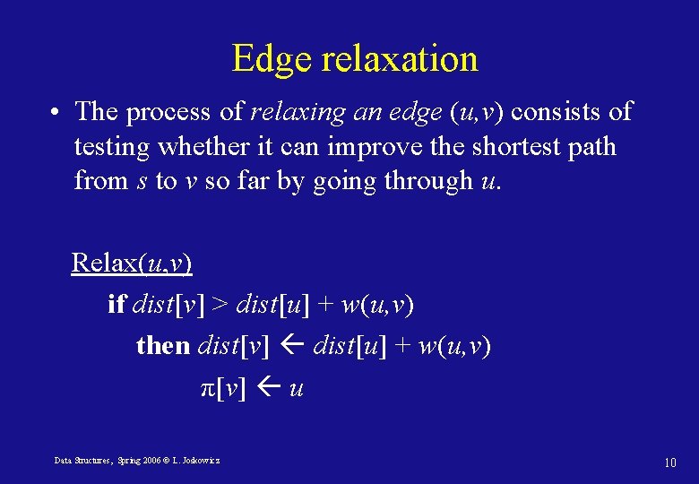
Edge relaxation • The process of relaxing an edge (u, v) consists of testing whether it can improve the shortest path from s to v so far by going through u. Relax(u, v) if dist[v] > dist[u] + w(u, v) then dist[v] dist[u] + w(u, v) π[v] u Data Structures, Spring 2006 © L. Joskowicz 10

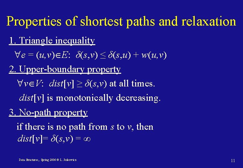
Properties of shortest paths and relaxation 1. Triangle inequality e = (u, v) E: δ(s, v) ≤ δ(s, u) + w(u, v) 2. Upper-boundary property v V: dist[v] ≥ δ(s, v) at all times. dist[v] is monotonically decreasing. 3. No-path property if there is no path from s to v, then dist[v]= δ(s, v) = ∞ Data Structures, Spring 2006 © L. Joskowicz 11

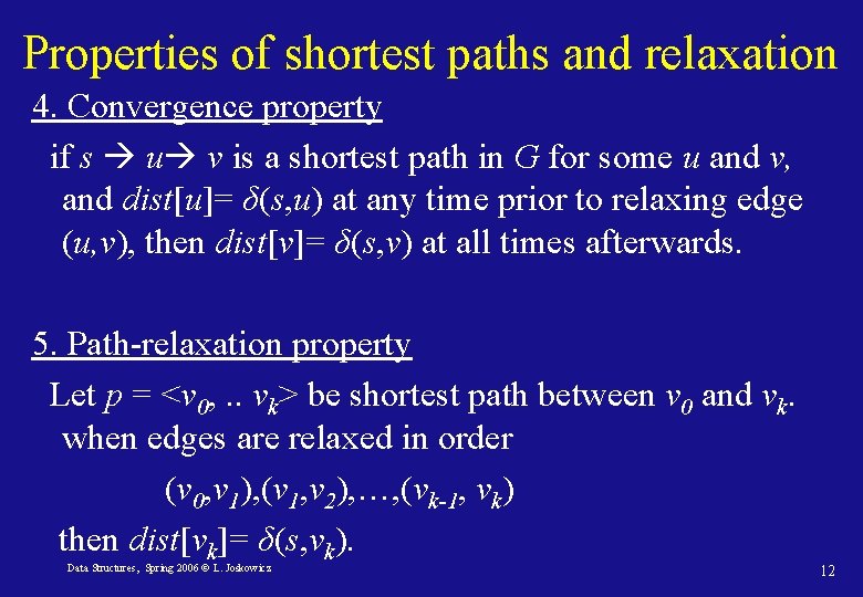
Properties of shortest paths and relaxation 4. Convergence property if s u v is a shortest path in G for some u and v, and dist[u]= δ(s, u) at any time prior to relaxing edge (u, v), then dist[v]= δ(s, v) at all times afterwards. 5. Path-relaxation property Let p = <v 0, . . vk> be shortest path between v 0 and vk. when edges are relaxed in order (v 0, v 1), (v 1, v 2), …, (vk-1, vk) then dist[vk]= δ(s, vk). Data Structures, Spring 2006 © L. Joskowicz 12

Properties of shortest paths and relaxation 6. Predecessor sub-graph property Once dist[v]= δ(s, v) for all v V, the predecessor subgraph is a shortest-paths tree rooted at s. Data Structures, Spring 2006 © L. Joskowicz 13

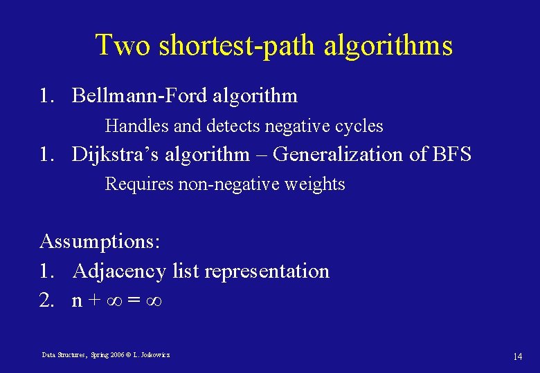
Two shortest-path algorithms 1. Bellmann-Ford algorithm Handles and detects negative cycles 1. Dijkstra’s algorithm – Generalization of BFS Requires non-negative weights Assumptions: 1. Adjacency list representation 2. n + ∞ = ∞ Data Structures, Spring 2006 © L. Joskowicz 14

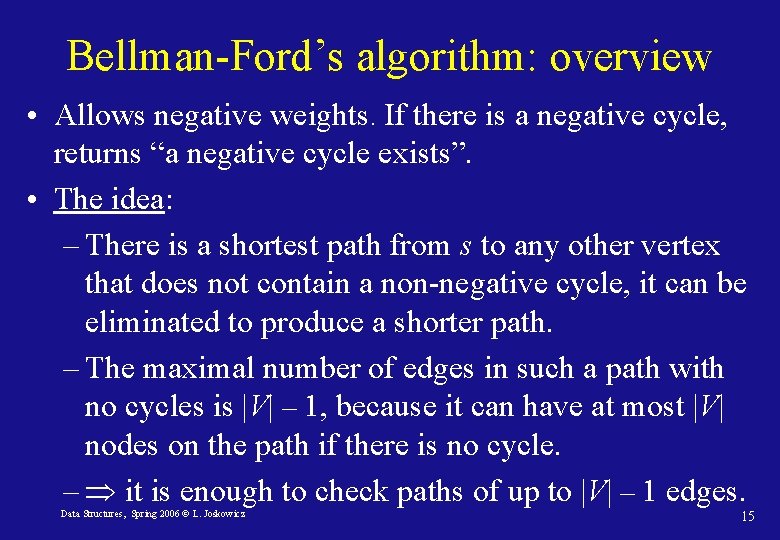
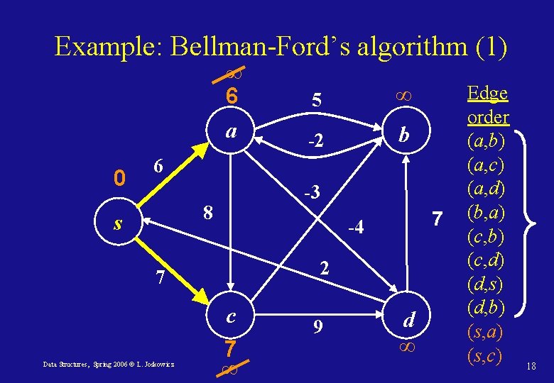
Bellman-Ford’s algorithm: overview • Allows negative weights. If there is a negative cycle, returns “a negative cycle exists”. • The idea: – There is a shortest path from s to any other vertex that does not contain a non-negative cycle, it can be eliminated to produce a shorter path. – The maximal number of edges in such a path with no cycles is |V| – 1, because it can have at most |V| nodes on the path if there is no cycle. – it is enough to check paths of up to |V| – 1 edges. Data Structures, Spring 2006 © L. Joskowicz 15

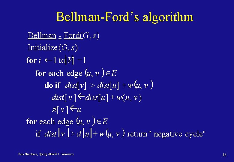
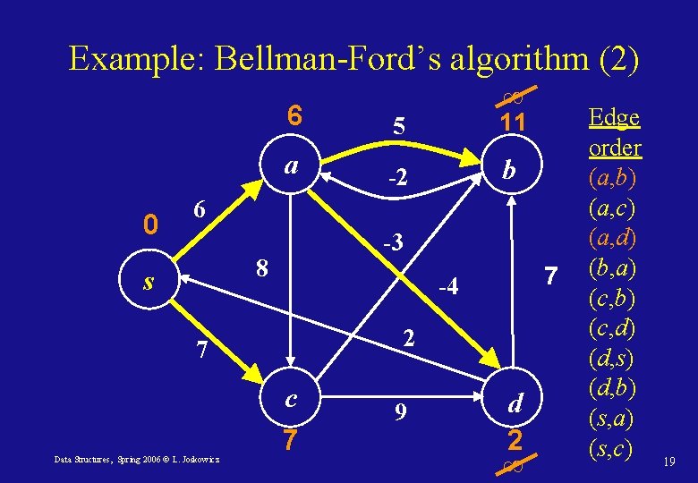
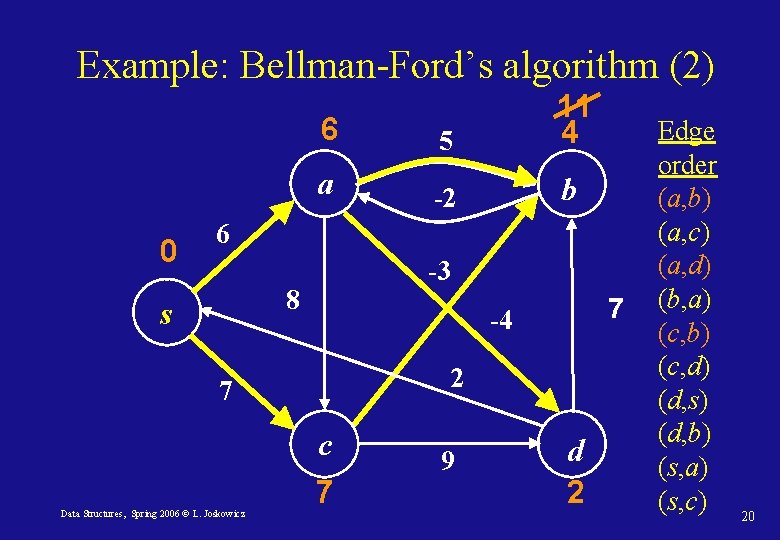
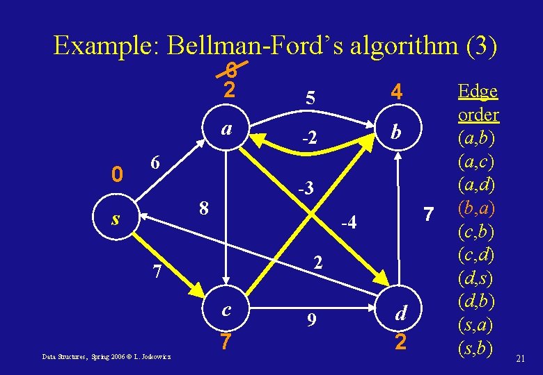
Bellman-Ford’s algorithm Bellman - Ford( G , s ) Initialize ( G , s ) for i ¬ 1 to|V| -1 for each edge (u, v ) E do if dist[v] > dist[u] + w (u, v ) dist [ v ] dist [u ] + w ( u, v ) p[ v ] u for each edge (u, v ) E if dist [v ] > d [u] + w (u, v ) return " negative cycle" Data Structures, Spring 2006 © L. Joskowicz 16

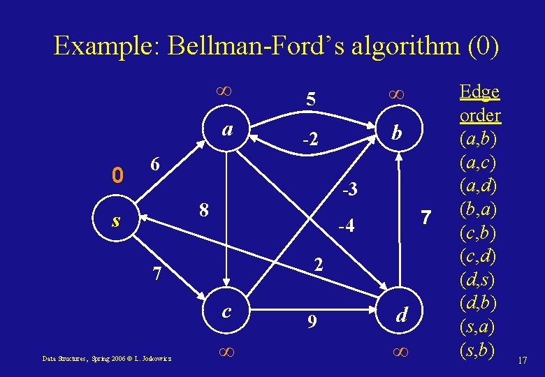
Example: Bellman-Ford’s algorithm (0) 0 ∞ 5 ∞ a -2 b 6 -3 8 s 2 7 c Data Structures, Spring 2006 © L. Joskowicz 7 -4 ∞ 9 d ∞ Edge order (a, b) (a, c) (a, d) (b, a) (c, b) (c, d) (d, s) (d, b) (s, a) (s, b) 17

Example: Bellman-Ford’s algorithm (1) 0 ∞ 6 5 ∞ a -2 b 6 -3 8 s 2 7 c Data Structures, Spring 2006 © L. Joskowicz 7 -4 7 ∞ 9 d ∞ Edge order (a, b) (a, c) (a, d) (b, a) (c, b) (c, d) (d, s) (d, b) (s, a) (s, c) 18

Example: Bellman-Ford’s algorithm (2) 0 ∞ 6 5 11 a -2 b 6 -3 8 s 2 7 c Data Structures, Spring 2006 © L. Joskowicz 7 -4 7 9 d 2 ∞ Edge order (a, b) (a, c) (a, d) (b, a) (c, b) (c, d) (d, s) (d, b) (s, a) (s, c) 19

Example: Bellman-Ford’s algorithm (2) 0 6 5 11 4 a -2 b 6 -3 8 s 2 7 c Data Structures, Spring 2006 © L. Joskowicz 7 -4 7 9 d 2 Edge order (a, b) (a, c) (a, d) (b, a) (c, b) (c, d) (d, s) (d, b) (s, a) (s, c) 20

Example: Bellman-Ford’s algorithm (3) 0 6 2 5 4 a -2 b 6 -3 8 s 2 7 c Data Structures, Spring 2006 © L. Joskowicz 7 -4 7 9 d 2 Edge order (a, b) (a, c) (a, d) (b, a) (c, b) (c, d) (d, s) (d, b) (s, a) (s, b) 21

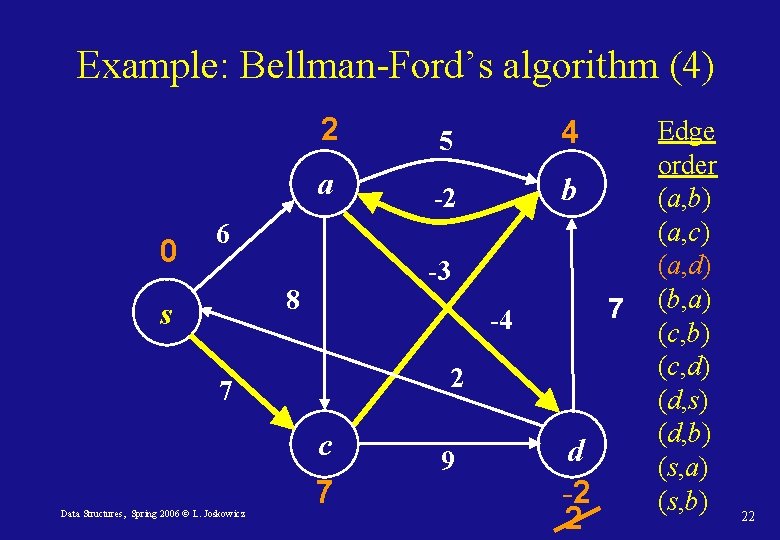
Example: Bellman-Ford’s algorithm (4) 0 2 5 4 a -2 b 6 -3 8 s 2 7 c Data Structures, Spring 2006 © L. Joskowicz 7 -4 7 9 d -2 2 Edge order (a, b) (a, c) (a, d) (b, a) (c, b) (c, d) (d, s) (d, b) (s, a) (s, b) 22

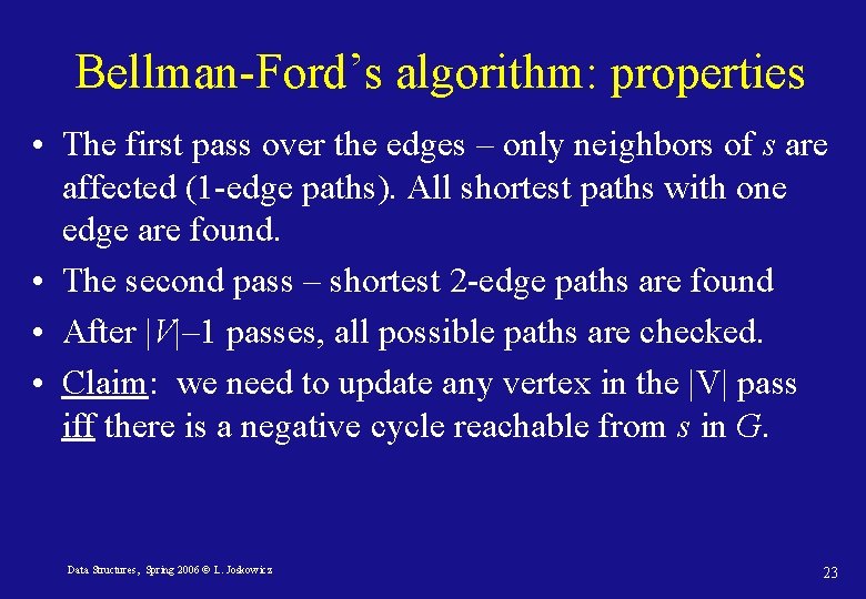
Bellman-Ford’s algorithm: properties • The first pass over the edges – only neighbors of s are affected (1 -edge paths). All shortest paths with one edge are found. • The second pass – shortest 2 -edge paths are found • After |V|– 1 passes, all possible paths are checked. • Claim: we need to update any vertex in the |V| pass iff there is a negative cycle reachable from s in G. Data Structures, Spring 2006 © L. Joskowicz 23

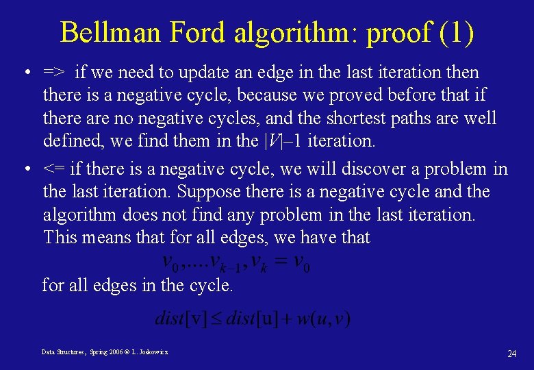
Bellman Ford algorithm: proof (1) • => if we need to update an edge in the last iteration there is a negative cycle, because we proved before that if there are no negative cycles, and the shortest paths are well defined, we find them in the |V|– 1 iteration. • <= if there is a negative cycle, we will discover a problem in the last iteration. Suppose there is a negative cycle and the algorithm does not find any problem in the last iteration. This means that for all edges, we have that for all edges in the cycle. Data Structures, Spring 2006 © L. Joskowicz 24

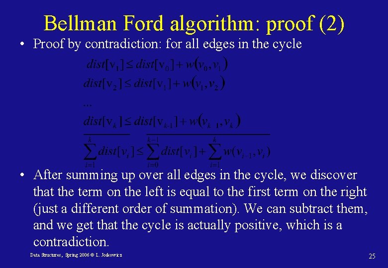
Bellman Ford algorithm: proof (2) • Proof by contradiction: for all edges in the cycle • After summing up over all edges in the cycle, we discover that the term on the left is equal to the first term on the right (just a different order of summation). We can subtract them, and we get that the cycle is actually positive, which is a contradiction. Data Structures, Spring 2006 © L. Joskowicz 25

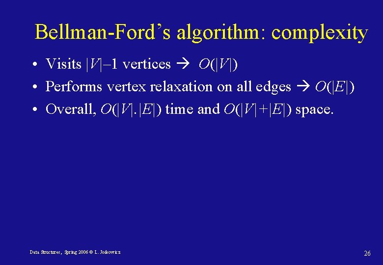
Bellman-Ford’s algorithm: complexity • Visits |V|– 1 vertices O(|V|) • Performs vertex relaxation on all edges O(|E|) • Overall, O(|V|. |E|) time and O(|V|+|E|) space. Data Structures, Spring 2006 © L. Joskowicz 26

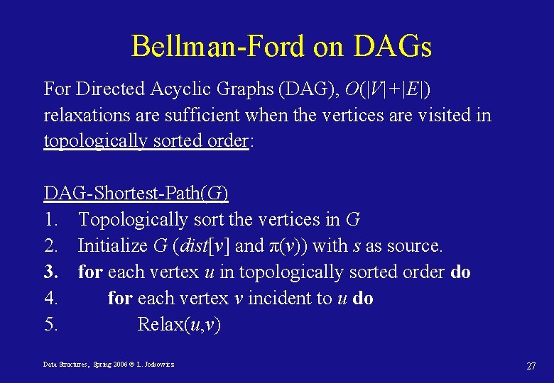
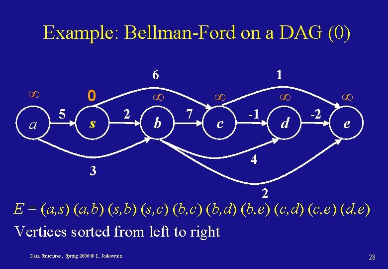
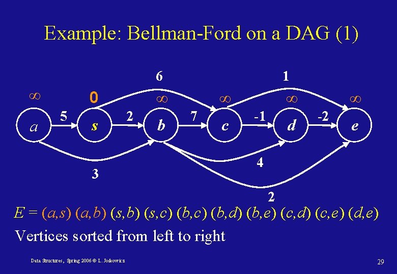
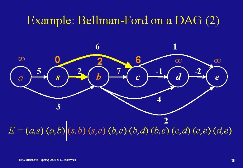
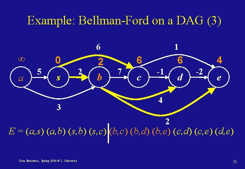
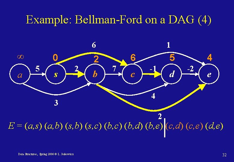
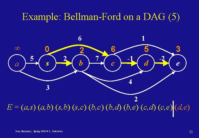
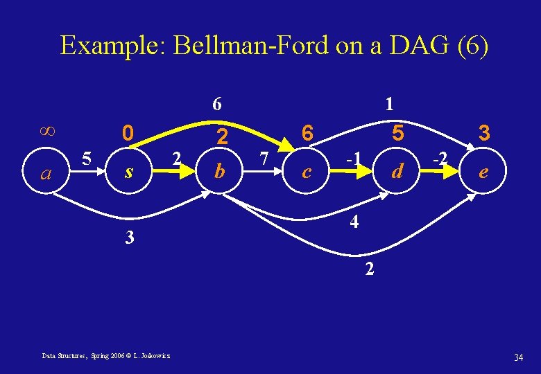
Bellman-Ford on DAGs For Directed Acyclic Graphs (DAG), O(|V|+|E|) relaxations are sufficient when the vertices are visited in topologically sorted order: DAG-Shortest-Path(G) 1. Topologically sort the vertices in G 2. Initialize G (dist[v] and π(v)) with s as source. 3. for each vertex u in topologically sorted order do 4. for each vertex v incident to u do 5. Relax(u, v) Data Structures, Spring 2006 © L. Joskowicz 27

Example: Bellman-Ford on a DAG (0) 6 ∞ a 0 5 s 3 1 ∞ 2 b ∞ 7 c ∞ -1 d ∞ -2 e 4 2 E = (a, s) (a, b) (s, c) (b, d) (b, e) (c, d) (c, e) (d, e) Vertices sorted from left to right Data Structures, Spring 2006 © L. Joskowicz 28

Example: Bellman-Ford on a DAG (1) 6 ∞ a 0 5 s 3 1 ∞ 2 b ∞ 7 c ∞ -1 d ∞ -2 e 4 2 E = (a, s) (a, b) (s, c) (b, d) (b, e) (c, d) (c, e) (d, e) Vertices sorted from left to right Data Structures, Spring 2006 © L. Joskowicz 29

Example: Bellman-Ford on a DAG (2) 6 ∞ a 0 5 s 3 2 2 b 1 6 7 c ∞ -1 d ∞ -2 e 4 2 E = (a, s) (a, b) (s, c) (b, d) (b, e) (c, d) (c, e) (d, e) Data Structures, Spring 2006 © L. Joskowicz 30

Example: Bellman-Ford on a DAG (3) 6 ∞ a 0 5 s 3 2 2 b 1 6 7 c 6 -1 d 4 -2 e 4 2 E = (a, s) (a, b) (s, c) (b, d) (b, e) (c, d) (c, e) (d, e) Data Structures, Spring 2006 © L. Joskowicz 31

Example: Bellman-Ford on a DAG (4) 6 ∞ a 0 5 s 3 2 2 b 1 6 7 c 5 -1 d 4 -2 e 4 2 E = (a, s) (a, b) (s, c) (b, d) (b, e) (c, d) (c, e) (d, e) Data Structures, Spring 2006 © L. Joskowicz 32

Example: Bellman-Ford on a DAG (5) 6 ∞ a 0 5 s 3 2 2 b 1 6 7 c 5 -1 d 3 -2 e 4 2 E = (a, s) (a, b) (s, c) (b, d) (b, e) (c, d) (c, e) (d, e) Data Structures, Spring 2006 © L. Joskowicz 33

Example: Bellman-Ford on a DAG (6) 6 ∞ a 0 5 s 3 2 2 b 1 6 7 c 5 -1 d 3 -2 e 4 2 Data Structures, Spring 2006 © L. Joskowicz 34

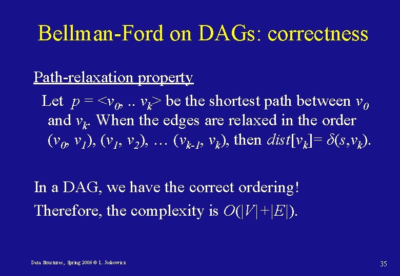
Bellman-Ford on DAGs: correctness Path-relaxation property Let p = <v 0, . . vk> be the shortest path between v 0 and vk. When the edges are relaxed in the order (v 0, v 1), (v 1, v 2), … (vk-1, vk), then dist[vk]= δ(s, vk). In a DAG, we have the correct ordering! Therefore, the complexity is O(|V|+|E|). Data Structures, Spring 2006 © L. Joskowicz 35

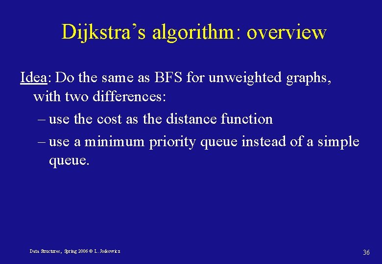
Dijkstra’s algorithm: overview Idea: Do the same as BFS for unweighted graphs, with two differences: – use the cost as the distance function – use a minimum priority queue instead of a simple queue. Data Structures, Spring 2006 © L. Joskowicz 36

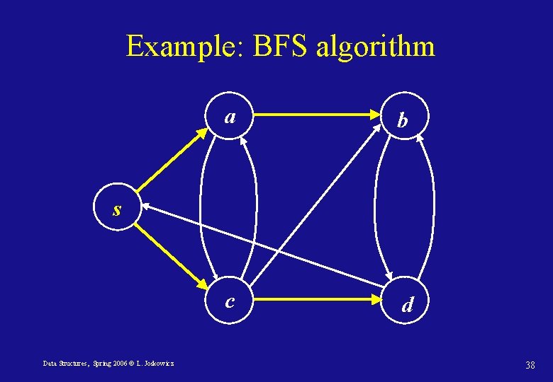
BFS(G, s) The BFS algorithm label[s] current; dist[s] = 0; π[s] = null for all vertices u in V – {s} do label[u] not_visited; dist[u] = ∞; π[u] = null En. Queue(Q, s) while Q is not empty do u De. Queue(Q) for each v that is a neighbor of u do if label[v] = not_visited then label[v] current dist[v] dist[u] + 1; π[v] u En. Queue(Q, v) label[u] visited Data Structures, Spring 2006 © L. Joskowicz 37

Example: BFS algorithm a b c d s Data Structures, Spring 2006 © L. Joskowicz 38

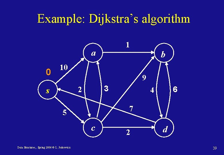
Example: Dijkstra’s algorithm 1 a 0 b 10 9 3 2 s 7 5 c Data Structures, Spring 2006 © L. Joskowicz 6 4 2 d 39

Dijkstra’s algorithm Dijkstra(G, s) label[s] current; dist[s] = 0; π[u] = null for all vertices u in V – {s} do label[u] not_visited; dist[u] = ∞; π[u] = null Q s while Q is not empty do u De. Queue(Q) Extract-Min(Q) for each v that is a neighbor of u do if label[v] = not_visited then label[v] current if d[v] > d[u] + w(u, v) then d[v] d[u] + w(u, v); π[v] = u Insert-Queue(Q, v) label[u] = visited Data Structures, Spring 2006 © L. Joskowicz 40

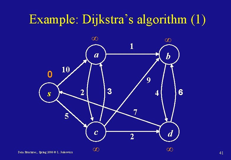
Example: Dijkstra’s algorithm (1) ∞ 1 a 0 ∞ b 10 9 3 2 s 7 5 c Data Structures, Spring 2006 © L. Joskowicz 6 4 ∞ 2 d ∞ 41

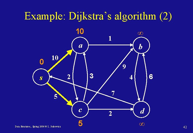
Example: Dijkstra’s algorithm (2) 10 1 a 0 ∞ b 10 9 3 2 s 7 5 c Data Structures, Spring 2006 © L. Joskowicz 6 4 5 2 d ∞ 42

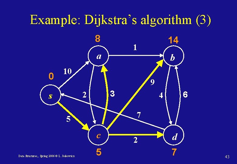
Example: Dijkstra’s algorithm (3) 8 1 a 0 14 b 10 9 3 2 s 7 5 c Data Structures, Spring 2006 © L. Joskowicz 6 4 5 2 d 7 43

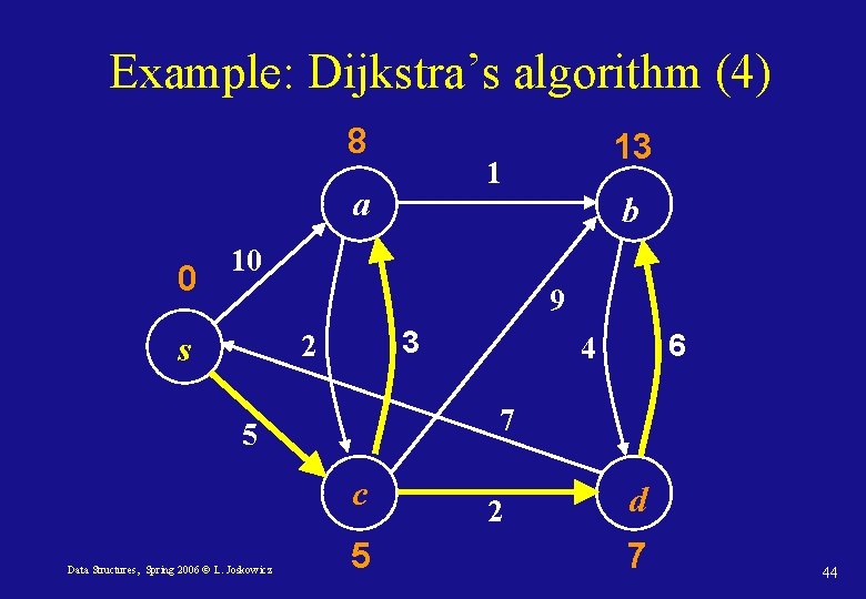
Example: Dijkstra’s algorithm (4) 8 1 a 0 13 b 10 9 3 2 s 7 5 c Data Structures, Spring 2006 © L. Joskowicz 6 4 5 2 d 7 44

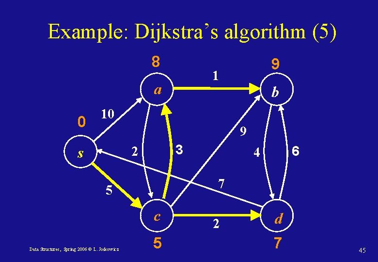
Example: Dijkstra’s algorithm (5) 8 1 a 0 9 b 10 9 3 2 s 7 5 c Data Structures, Spring 2006 © L. Joskowicz 6 4 5 2 d 7 45

Example: Dijkstra’s algorithm (6) 8 1 a 0 9 b 10 9 3 2 s 7 5 c Data Structures, Spring 2006 © L. Joskowicz 6 4 5 2 d 7 46

Dijkstra’s algorithm: correctness (1) Theorem: Upon termination of Dijkstra’s algorithm dist[v] = δ(s, v) for each vertex v V Definition: a path from s to v is said to be a special path if it is the shortest path from s to v in which all vertices (except maybe for v) are inside S. Lemma: At the end of each iteration of the while loop, the following two properties hold: 1. For each w S, dist[w] is the length of the shortest path from s to w which stays inside S. 2. For each w (V–S), dist(w) is the length of the shortest special path from s to w. The theorem follows when S = V. Data Structures, Spring 2006 © L. Joskowicz 47

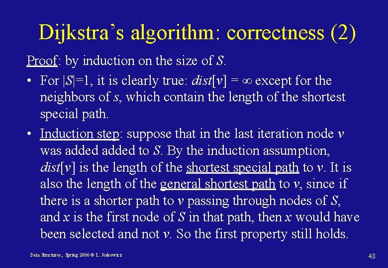
Dijkstra’s algorithm: correctness (2) Proof: by induction on the size of S. • For |S|=1, it is clearly true: dist[v] = ∞ except for the neighbors of s, which contain the length of the shortest special path. • Induction step: suppose that in the last iteration node v was added to S. By the induction assumption, dist[v] is the length of the shortest special path to v. It is also the length of the general shortest path to v, since if there is a shorter path to v passing through nodes of S, and x is the first node of S in that path, then x would have been selected and not v. So the first property still holds. Data Structures, Spring 2006 © L. Joskowicz 48

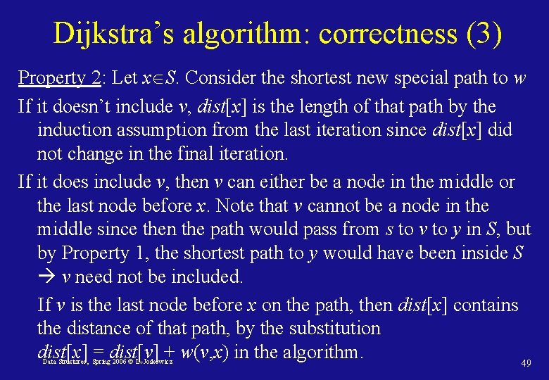
Dijkstra’s algorithm: correctness (3) Property 2: Let x S. Consider the shortest new special path to w If it doesn’t include v, dist[x] is the length of that path by the induction assumption from the last iteration since dist[x] did not change in the final iteration. If it does include v, then v can either be a node in the middle or the last node before x. Note that v cannot be a node in the middle since then the path would pass from s to v to y in S, but by Property 1, the shortest path to y would have been inside S v need not be included. If v is the last node before x on the path, then dist[x] contains the distance of that path, by the substitution dist[x] = dist[v] + w(v, x) in the algorithm. 49 Data Structures, Spring 2006 © L. Joskowicz

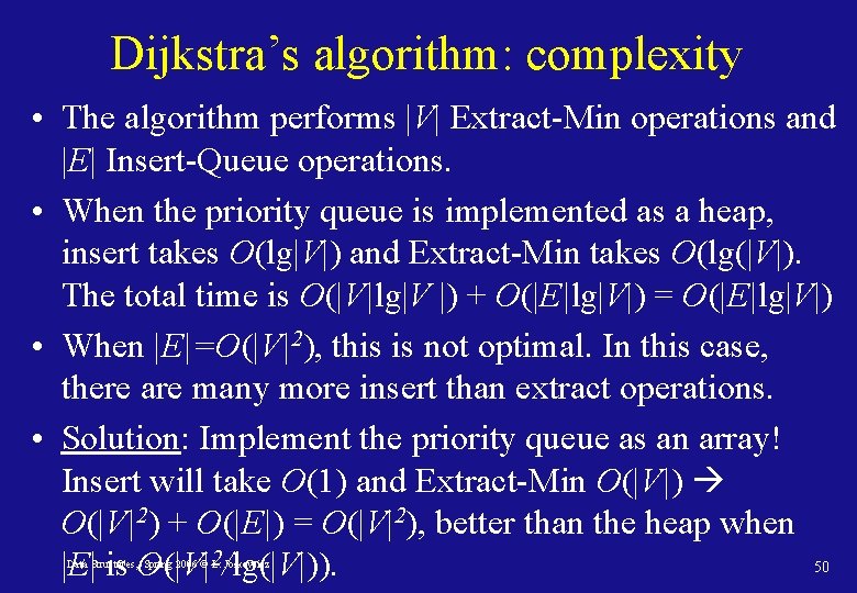
Dijkstra’s algorithm: complexity • The algorithm performs |V| Extract-Min operations and |E| Insert-Queue operations. • When the priority queue is implemented as a heap, insert takes O(lg|V|) and Extract-Min takes O(lg(|V|). The total time is O(|V|lg|V |) + O(|E|lg|V|) = O(|E|lg|V|) • When |E|=O(|V|2), this is not optimal. In this case, there are many more insert than extract operations. • Solution: Implement the priority queue as an array! Insert will take O(1) and Extract-Min O(|V|) O(|V|2) + O(|E|) = O(|V|2), better than the heap when 50 |E| is O(|V|2/lg(|V|)). Data Structures, Spring 2006 © L. Joskowicz

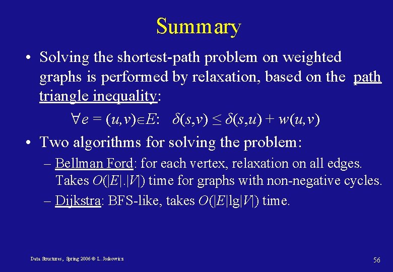
Summary • Solving the shortest-path problem on weighted graphs is performed by relaxation, based on the path triangle inequality: e = (u, v) E: δ(s, v) ≤ δ(s, u) + w(u, v) • Two algorithms for solving the problem: – Bellman Ford: for each vertex, relaxation on all edges. Takes O(|E|. |V|) time for graphs with non-negative cycles. – Dijkstra: BFS-like, takes O(|E|lg|V|) time. Data Structures, Spring 2006 © L. Joskowicz 56