Data Structures LECTURE 10 Huffman coding Motivation Uniquely

Data Structures – LECTURE 10 Huffman coding • • • Motivation Uniquely decipherable codes Prefix codes Huffman code construction Extensions and applications Chapter 16. 3 pp 385— 392 in textbook Data Structures, Spring 2004 © L. Joskowicz 1

Motivation • Suppose we want to store and transmit very large files (messages) consisting of strings (words) constructed over an alphabet of characters (letters). • Representing each character with a fixed-length code will not result in the shortest possible file! • Example: 8 -bit ASCII code for characters – some characters are much more frequent than others – using shorter codes for frequent characters and longer ones for infrequent ones will result in a shorter file Data Structures, Spring 2004 © L. Joskowicz 2

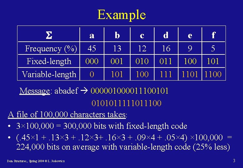
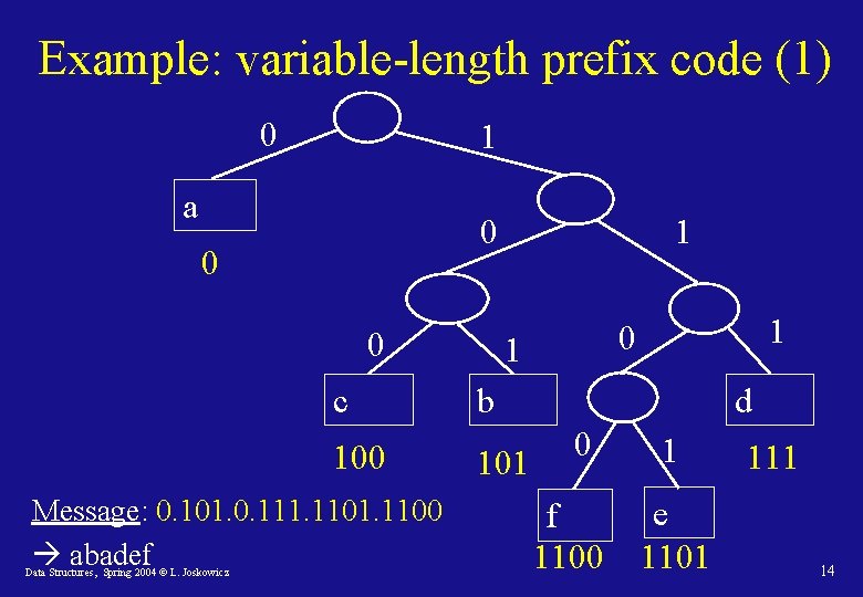
Example a Frequency (%) 45 Fixed-length 000 Variable-length 0 b c 13 001 12 010 100 d e f 16 9 5 011 100 101 1101 1100 Message: abadef 000001110010101111100 A file of 100, 000 characters takes: • 3× 100, 000 = 300, 000 bits with fixed-length code • (. 45× 1 +. 13× 3 +. 12× 3+. 16× 3 +. 09× 4 +. 05× 4) × 100, 000 = 224, 000 bits on average with variable-length code (25% less) Data Structures, Spring 2004 © L. Joskowicz 3

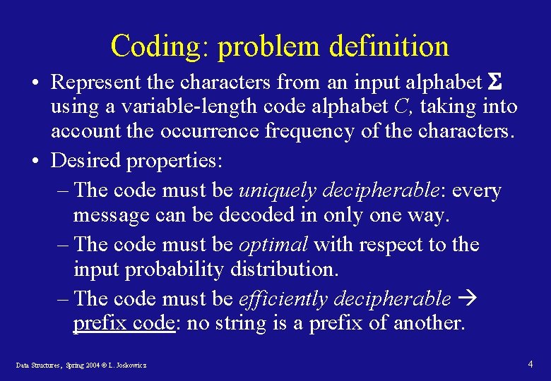
Coding: problem definition • Represent the characters from an input alphabet using a variable-length code alphabet C, taking into account the occurrence frequency of the characters. • Desired properties: – The code must be uniquely decipherable: every message can be decoded in only one way. – The code must be optimal with respect to the input probability distribution. – The code must be efficiently decipherable prefix code: no string is a prefix of another. Data Structures, Spring 2004 © L. Joskowicz 4

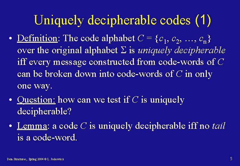
Uniquely decipherable codes (1) • Definition: The code alphabet C = {c 1, c 2, …, cn} over the original alphabet is uniquely decipherable iff every message constructed from code-words of C can be broken down into code-words of C in only one way. • Question: how can we test if C is uniquely decipherable? • Lemma: a code C is uniquely decipherable iff no tail is a code-word. Data Structures, Spring 2004 © L. Joskowicz 5

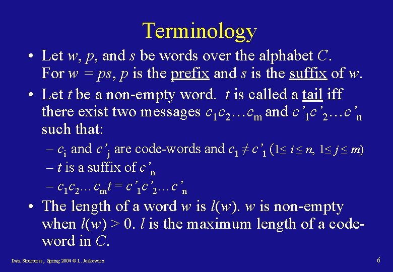
Terminology • Let w, p, and s be words over the alphabet C. For w = ps, p is the prefix and s is the suffix of w. • Let t be a non-empty word. t is called a tail iff there exist two messages c 1 c 2…cm and c’ 1 c’ 2…c’n such that: – ci and c’j are code-words and c 1 ≠ c’ 1 (1≤ i ≤ n, 1≤ j ≤ m) – t is a suffix of c’n – c 1 c 2…cmt = c’ 1 c’ 2…c’n • The length of a word w is l(w). w is non-empty when l(w) > 0. l is the maximum length of a codeword in C. Data Structures, Spring 2004 © L. Joskowicz 6

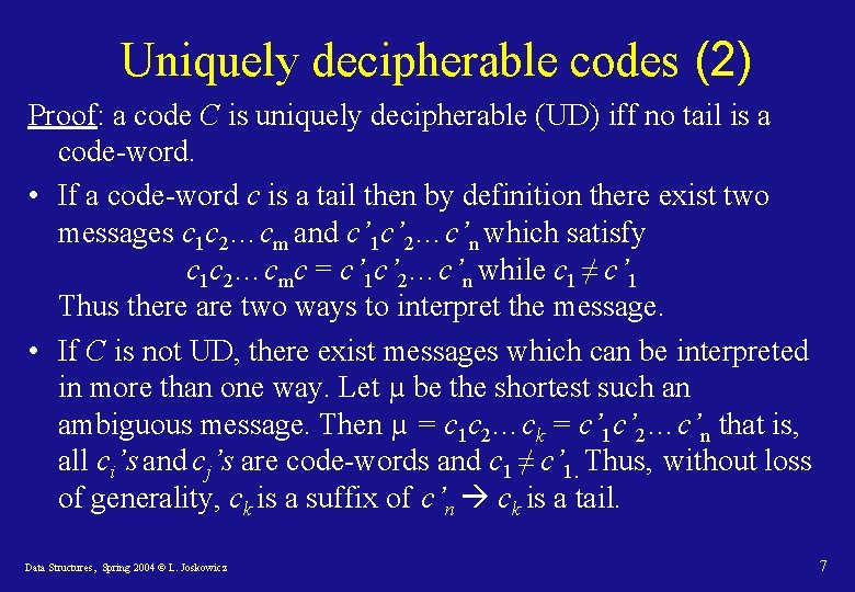
Uniquely decipherable codes (2) Proof: a code C is uniquely decipherable (UD) iff no tail is a code-word. • If a code-word c is a tail then by definition there exist two messages c 1 c 2…cm and c’ 1 c’ 2…c’n which satisfy c 1 c 2…cmc = c’ 1 c’ 2…c’n while c 1 ≠ c’ 1 Thus there are two ways to interpret the message. • If C is not UD, there exist messages which can be interpreted in more than one way. Let µ be the shortest such an ambiguous message. Then µ = c 1 c 2…ck = c’ 1 c’ 2…c’n that is, all ci’s and cj’s are code-words and c 1 ≠ c’ 1. Thus, without loss of generality, ck is a suffix of c’n ck is a tail. Data Structures, Spring 2004 © L. Joskowicz 7

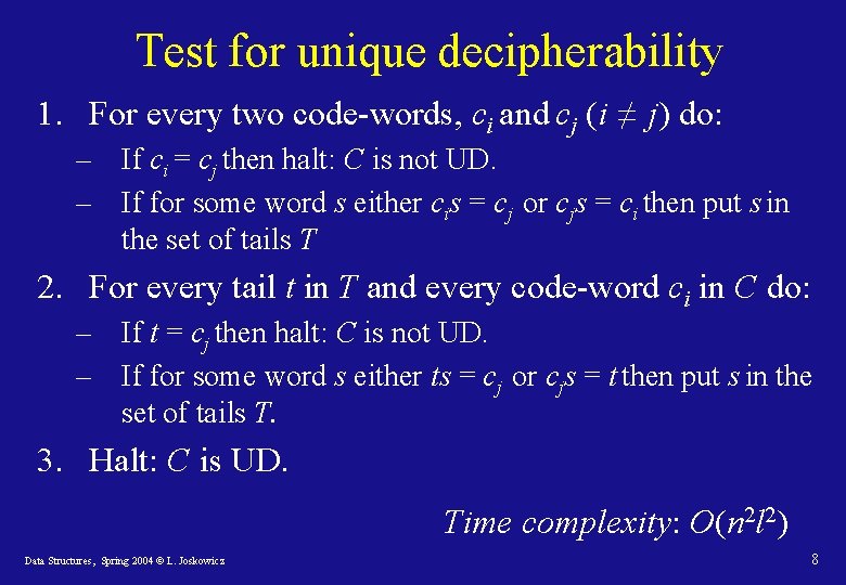
Test for unique decipherability 1. For every two code-words, ci and cj (i ≠ j) do: – If ci = cj then halt: C is not UD. – If for some word s either cis = cj or cjs = ci then put s in the set of tails T 2. For every tail t in T and every code-word ci in C do: – If t = cj then halt: C is not UD. – If for some word s either ts = cj or cjs = t then put s in the set of tails T. 3. Halt: C is UD. Time complexity: O(n 2 l 2) Data Structures, Spring 2004 © L. Joskowicz 8

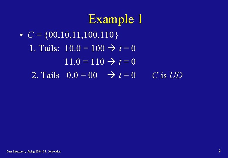
Example 1 • C = {00, 11, 100, 110} 1. Tails: 10. 0 = 100 t = 0 11. 0 = 110 t = 0 2. Tails 0. 0 = 00 t = 0 Data Structures, Spring 2004 © L. Joskowicz C is UD 9

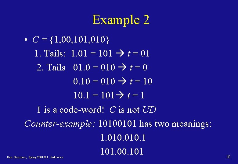
Example 2 • C = {1, 00, 101, 010} 1. Tails: 1. 01 = 101 t = 01 2. Tails 01. 0 = 010 t = 0 0. 10 = 010 t = 10 10. 1 = 101 t = 1 1 is a code-word! C is not UD Counter-example: 10100101 has two meanings: 1. 010. 1 101. 00. 101 Data Structures, Spring 2004 © L. Joskowicz 10

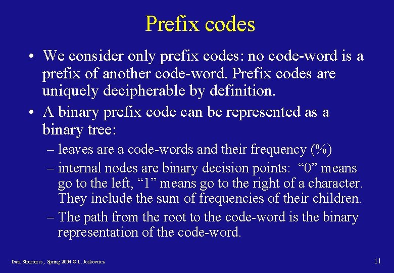
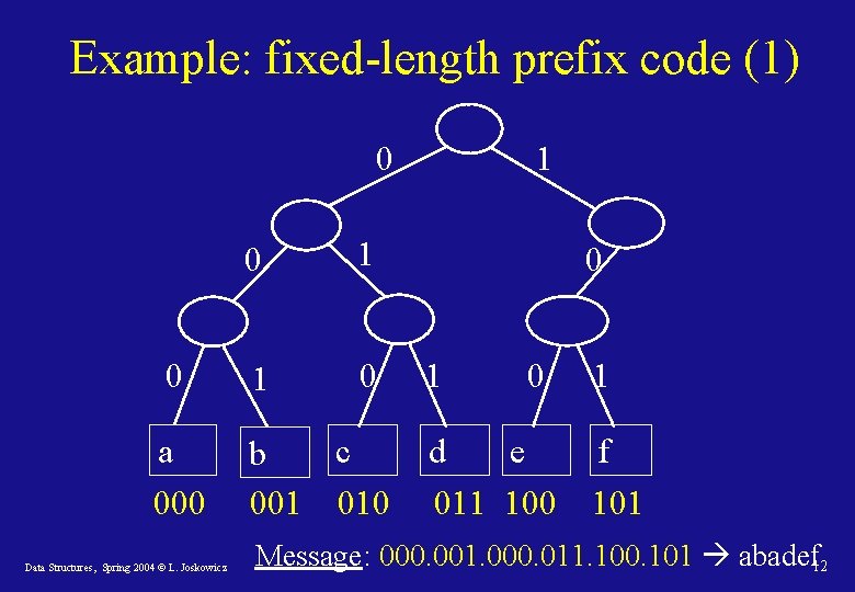
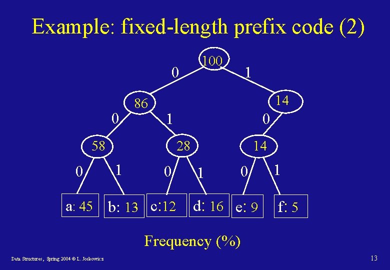
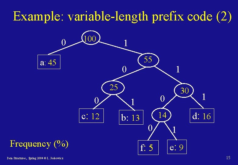
Prefix codes • We consider only prefix codes: no code-word is a prefix of another code-word. Prefix codes are uniquely decipherable by definition. • A binary prefix code can be represented as a binary tree: – leaves are a code-words and their frequency (%) – internal nodes are binary decision points: “ 0” means go to the left, “ 1” means go to the right of a character. They include the sum of frequencies of their children. – The path from the root to the code-word is the binary representation of the code-word. Data Structures, Spring 2004 © L. Joskowicz 11

Example: fixed-length prefix code (1) 0 0 a 000 Data Structures, Spring 2004 © L. Joskowicz 0 1 1 0 c b 001 010 1 0 d e 011 100 1 f 101 Message: 000. 001. 000. 011. 100. 101 abadef 12

Example: fixed-length prefix code (2) 0 0 86 1 14 1 58 0 100 0 28 1 0 a: 45 b: 13 c: 12 14 1 0 d: 16 e: 9 1 f: 5 Frequency (%) Data Structures, Spring 2004 © L. Joskowicz 13

Example: variable-length prefix code (1) 0 1 a 0 0 0 c 100 Message: 0. 101. 0. 111. 1100 abadef Data Structures, Spring 2004 © L. Joskowicz 1 1 0 1 b 101 d 0 f 1100 1 e 1101 111 14

Example: variable-length prefix code (2) 0 100 1 a: 45 55 0 1 25 0 c: 12 Frequency (%) Data Structures, Spring 2004 © L. Joskowicz 1 0 b: 13 14 0 f: 5 30 1 d: 16 1 e: 9 15

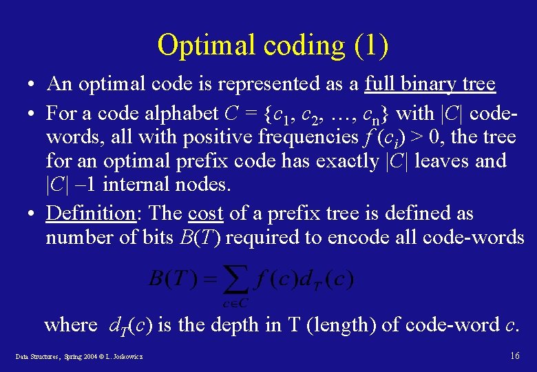
Optimal coding (1) • An optimal code is represented as a full binary tree • For a code alphabet C = {c 1, c 2, …, cn} with |C| codewords, all with positive frequencies f (ci) > 0, the tree for an optimal prefix code has exactly |C| leaves and |C| – 1 internal nodes. • Definition: The cost of a prefix tree is defined as number of bits B(T) required to encode all code-words where d. T(c) is the depth in T (length) of code-word c. Data Structures, Spring 2004 © L. Joskowicz 16

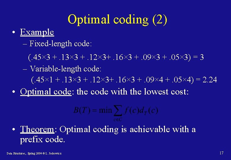
Optimal coding (2) • Example – Fixed-length code: (. 45× 3 +. 13× 3 +. 12× 3+. 16× 3 +. 09× 3 +. 05× 3) = 3 – Variable-length code: (. 45× 1 +. 13× 3 +. 12× 3+. 16× 3 +. 09× 4 +. 05× 4) = 2. 24 • Optimal code: the code with the lowest cost: • Theorem: Optimal coding is achievable with a prefix code. Data Structures, Spring 2004 © L. Joskowicz 17

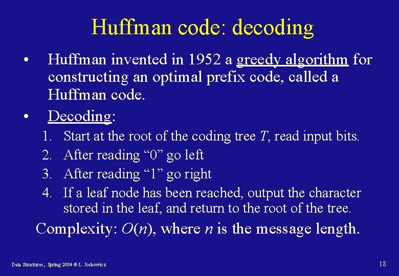
Huffman code: decoding • • Huffman invented in 1952 a greedy algorithm for constructing an optimal prefix code, called a Huffman code. Decoding: 1. 2. 3. 4. Start at the root of the coding tree T, read input bits. After reading “ 0” go left After reading “ 1” go right If a leaf node has been reached, output the character stored in the leaf, and return to the root of the tree. Complexity: O(n), where n is the message length. Data Structures, Spring 2004 © L. Joskowicz 18

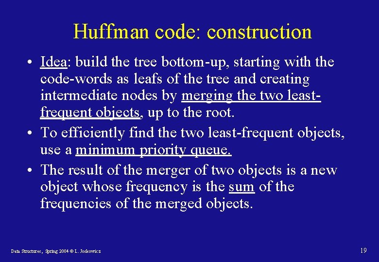
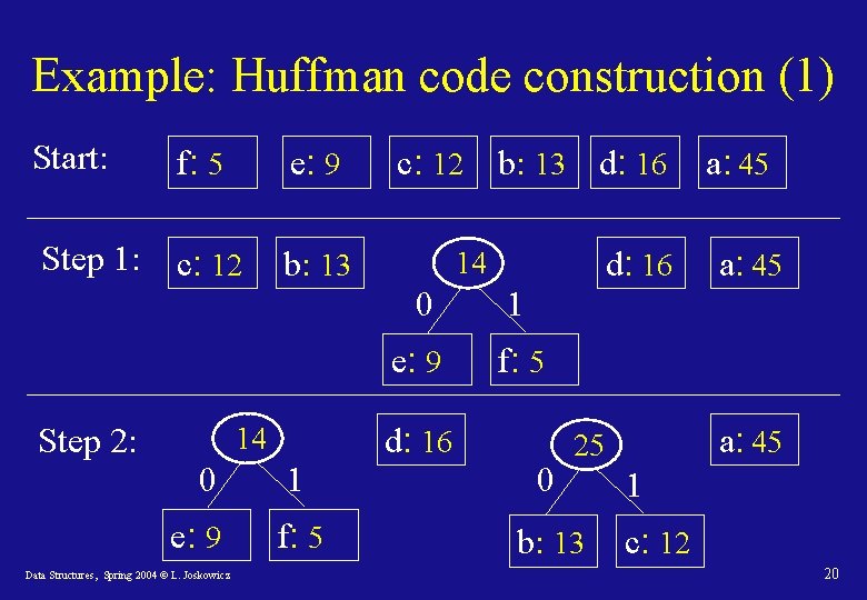
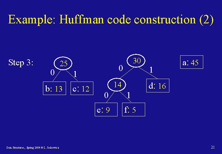
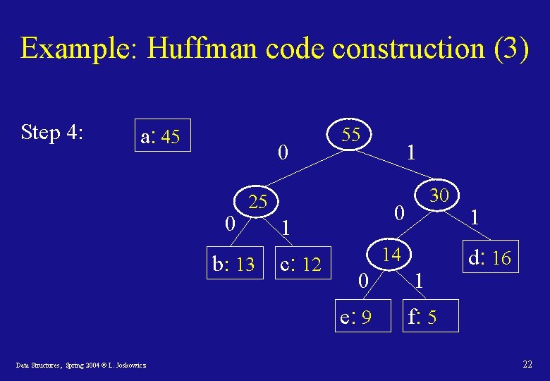
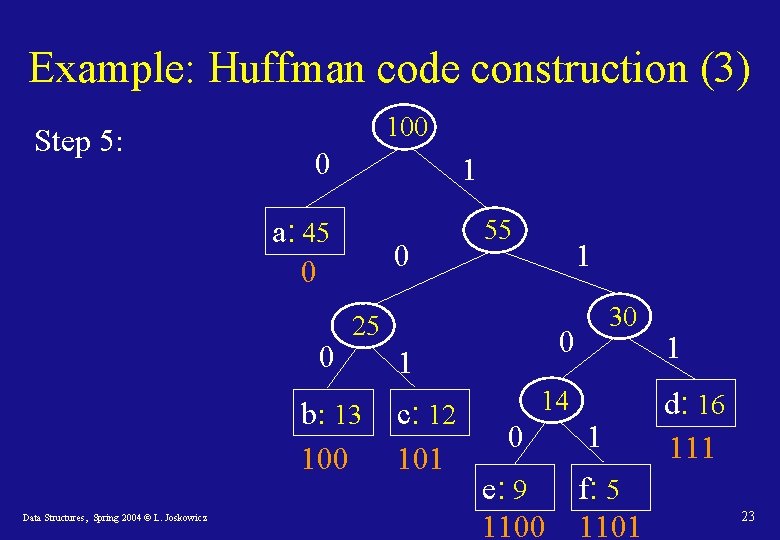
Huffman code: construction • Idea: build the tree bottom-up, starting with the code-words as leafs of the tree and creating intermediate nodes by merging the two leastfrequent objects, up to the root. • To efficiently find the two least-frequent objects, use a minimum priority queue. • The result of the merger of two objects is a new object whose frequency is the sum of the frequencies of the merged objects. Data Structures, Spring 2004 © L. Joskowicz 19

Example: Huffman code construction (1) Start: f: 5 e: 9 Step 1: c: 12 b: 13 Step 2: 14 0 e: 9 Data Structures, Spring 2004 © L. Joskowicz 1 f: 5 c: 12 b: 13 d: 16 14 0 1 e: 9 f: 5 d: 16 0 a: 45 25 b: 13 a: 45 1 c: 12 20

Example: Huffman code construction (2) Step 3: 0 25 b: 13 0 1 c: 12 14 0 e: 9 Data Structures, Spring 2004 © L. Joskowicz 30 1 1 a: 45 d: 16 f: 5 21

Example: Huffman code construction (3) Step 4: a: 45 0 0 55 25 b: 13 14 0 e: 9 Data Structures, Spring 2004 © L. Joskowicz 30 0 1 c: 12 1 1 1 d: 16 f: 5 22

Example: Huffman code construction (3) Step 5: 100 0 1 a: 45 0 0 0 1 25 b: 13 100 Data Structures, Spring 2004 © L. Joskowicz 55 0 1 c: 12 101 30 14 0 e: 9 1100 1 f: 5 1101 1 d: 16 111 23

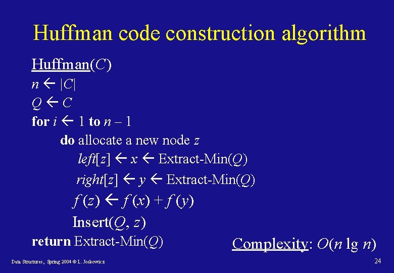
Huffman code construction algorithm Huffman(C) n |C| Q C for i 1 to n – 1 do allocate a new node z left[z] x Extract-Min(Q) right[z] y Extract-Min(Q) f (z) f (x) + f (y) Insert(Q, z) return Extract-Min(Q) Data Structures, Spring 2004 © L. Joskowicz Complexity: O(n lg n) 24

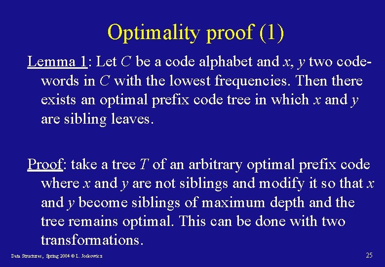
Optimality proof (1) Lemma 1: Let C be a code alphabet and x, y two codewords in C with the lowest frequencies. Then there exists an optimal prefix code tree in which x and y are sibling leaves. Proof: take a tree T of an arbitrary optimal prefix code where x and y are not siblings and modify it so that x and y become siblings of maximum depth and the tree remains optimal. This can be done with two transformations. Data Structures, Spring 2004 © L. Joskowicz 25

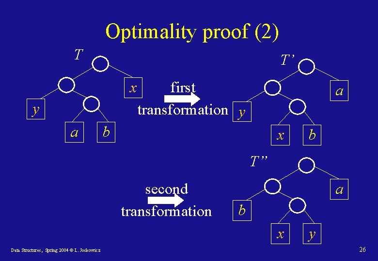
Optimality proof (2) T T’ x y a first transformation y a b x b T” second transformation a b x Data Structures, Spring 2004 © L. Joskowicz y 26

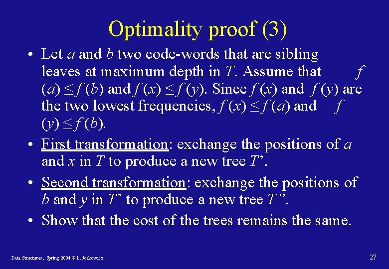
Optimality proof (3) • Let a and b two code-words that are sibling leaves at maximum depth in T. Assume that f (a) ≤ f (b) and f (x) ≤ f (y). Since f (x) and f (y) are the two lowest frequencies, f (x) ≤ f (a) and f (y) ≤ f (b). • First transformation: exchange the positions of a and x in T to produce a new tree T’. • Second transformation: exchange the positions of b and y in T’ to produce a new tree T”. • Show that the cost of the trees remains the same. Data Structures, Spring 2004 © L. Joskowicz 27

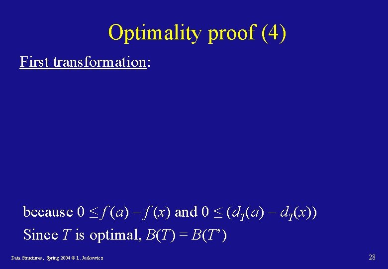
Optimality proof (4) First transformation: because 0 ≤ f (a) – f (x) and 0 ≤ (d. T(a) – d. T(x)) Since T is optimal, B(T) = B(T’) Data Structures, Spring 2004 © L. Joskowicz 28

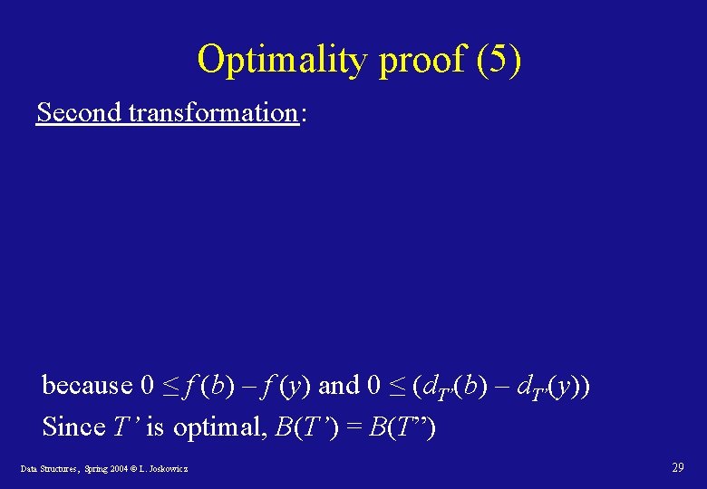
Optimality proof (5) Second transformation: because 0 ≤ f (b) – f (y) and 0 ≤ (d. T’(b) – d. T’(y)) Since T’ is optimal, B(T’) = B(T”) Data Structures, Spring 2004 © L. Joskowicz 29

Conclusion from Lemma 1 • Building up an optimal tree by mergers can begin with the greedy choice of merging together the two code-words with the lowest frequencies. • This is a greedy choice since the cost of a single merger is the sum of the lowest frequencies, which is the least expensive merge. Data Structures, Spring 2004 © L. Joskowicz 30

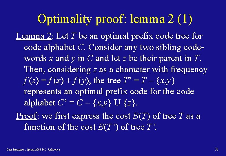
Optimality proof: lemma 2 (1) Lemma 2: Let T be an optimal prefix code tree for code alphabet C. Consider any two sibling codewords x and y in C and let z be their parent in T. Then, considering z as a character with frequency f (z) = f (x) + f (y), the tree T’ = T – {x, y} represents an optimal prefix code for the code alphabet C’ = C – {x, y} U {z}. Proof: we first express the cost B(T) of tree T as a function of the cost B(T’) of tree T’. Data Structures, Spring 2004 © L. Joskowicz 31

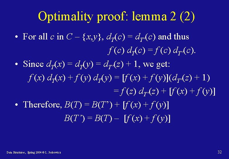
Optimality proof: lemma 2 (2) • For all c in C – {x, y}, d. T(c) = d. T’(c) and thus f (c) d. T(c) = f (c) d. T’(c). • Since d. T(x) = d. T(y) = d. T’(z) + 1, we get: f (x) d. T(x) + f (y) d. T(y) = [f (x) + f (y)](d. T’(z) + 1) = f (z) d. T’(z) + [f (x) + f (y)] • Therefore, B(T) = B(T’) + [f (x) + f (y)] B(T’) = B(T) – [f (x) + f (y)] Data Structures, Spring 2004 © L. Joskowicz 32

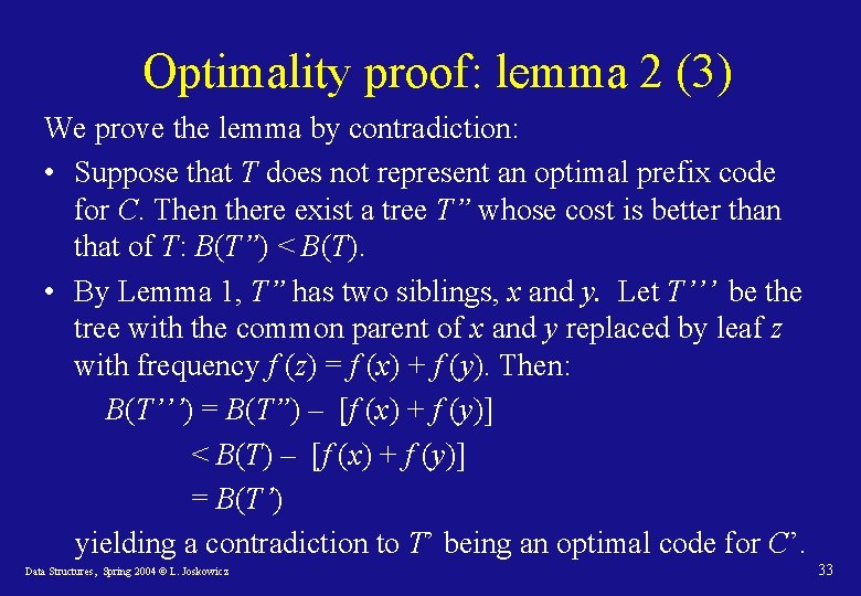
Optimality proof: lemma 2 (3) We prove the lemma by contradiction: • Suppose that T does not represent an optimal prefix code for C. Then there exist a tree T” whose cost is better than that of T: B(T”) < B(T). • By Lemma 1, T” has two siblings, x and y. Let T’’’ be the tree with the common parent of x and y replaced by leaf z with frequency f (z) = f (x) + f (y). Then: B(T’’’) = B(T”) – [f (x) + f (y)] < B(T) – [f (x) + f (y)] = B(T’) yielding a contradiction to T’ being an optimal code for C’. Data Structures, Spring 2004 © L. Joskowicz 33

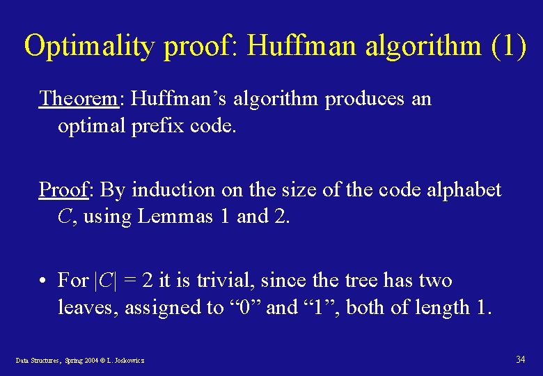
Optimality proof: Huffman algorithm (1) Theorem: Huffman’s algorithm produces an optimal prefix code. Proof: By induction on the size of the code alphabet C, using Lemmas 1 and 2. • For |C| = 2 it is trivial, since the tree has two leaves, assigned to “ 0” and “ 1”, both of length 1. Data Structures, Spring 2004 © L. Joskowicz 34

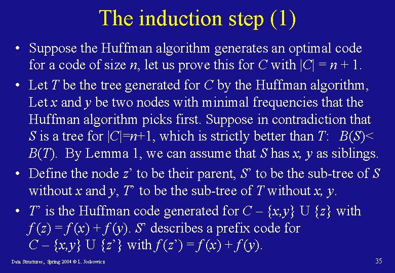
The induction step (1) • Suppose the Huffman algorithm generates an optimal code for a code of size n, let us prove this for C with |C| = n + 1. • Let T be the tree generated for C by the Huffman algorithm, Let x and y be two nodes with minimal frequencies that the Huffman algorithm picks first. Suppose in contradiction that S is a tree for |C|=n+1, which is strictly better than T: B(S)< B(T). By Lemma 1, we can assume that S has x, y as siblings. • Define the node z’ to be their parent, S’ to be the sub-tree of S without x and y, T’ to be the sub-tree of T without x, y. • T’ is the Huffman code generated for C – {x, y} U {z} with f (z) = f (x) + f (y). S’ describes a prefix code for C – {x, y} U {z’} with f (z’) = f (x) + f (y). Data Structures, Spring 2004 © L. Joskowicz 35

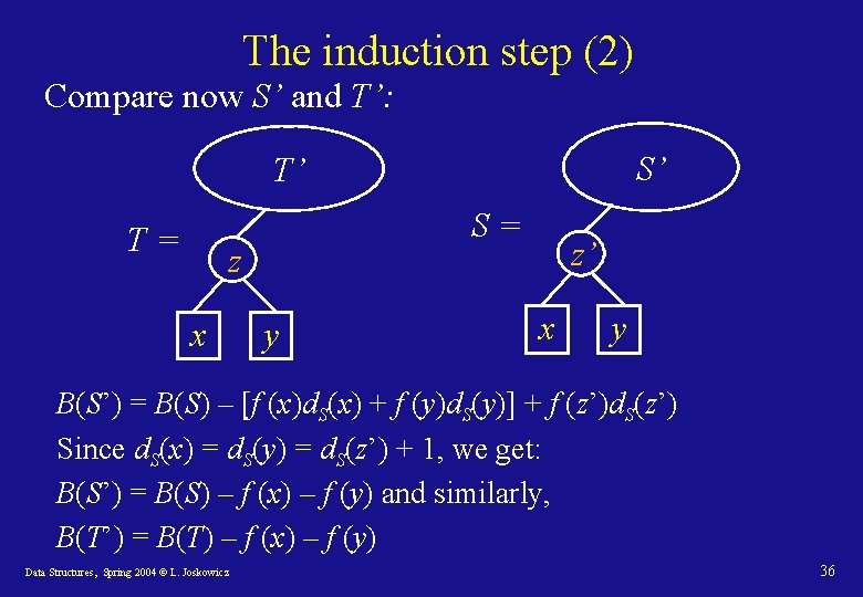
The induction step (2) Compare now S’ and T’: S’ T’ T= S= z x y z’ x y B(S’) = B(S) – [f (x)d. S(x) + f (y)d. S(y)] + f (z’)d. S(z’) Since d. S(x) = d. S(y) = d. S(z’) + 1, we get: B(S’) = B(S) – f (x) – f (y) and similarly, B(T’) = B(T) – f (x) – f (y) Data Structures, Spring 2004 © L. Joskowicz 36

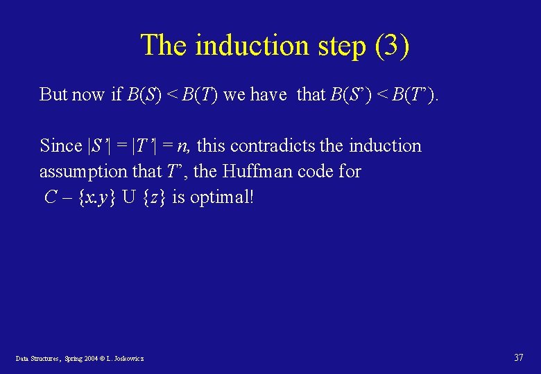
The induction step (3) But now if B(S) < B(T) we have that B(S’) < B(T’). Since |S’| = |T’| = n, this contradicts the induction assumption that T’, the Huffman code for C – {x. y} U {z} is optimal! Data Structures, Spring 2004 © L. Joskowicz 37

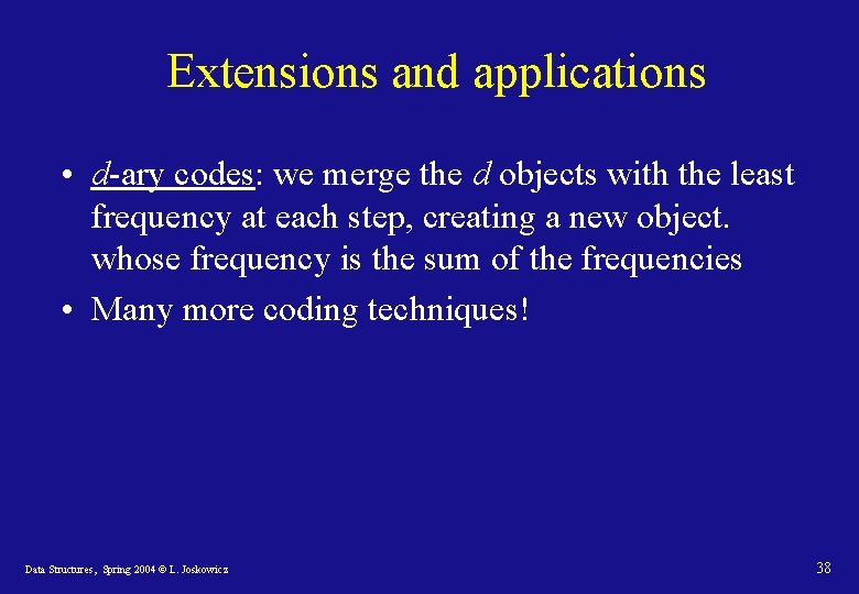
Extensions and applications • d-ary codes: we merge the d objects with the least frequency at each step, creating a new object. whose frequency is the sum of the frequencies • Many more coding techniques! Data Structures, Spring 2004 © L. Joskowicz 38