
Data Structures Dynamic Sets Heaps Binary Trees Sorting
Data Structures Dynamic Sets Heaps Binary Trees & Sorting Hashing
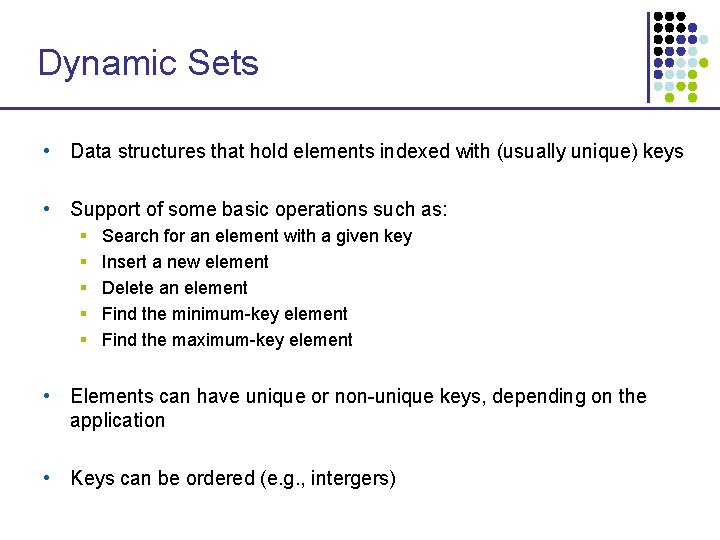
Dynamic Sets • Data structures that hold elements indexed with (usually unique) keys • Support of some basic operations such as: § § § Search for an element with a given key Insert a new element Delete an element Find the minimum-key element Find the maximum-key element • Elements can have unique or non-unique keys, depending on the application • Keys can be ordered (e. g. , intergers)
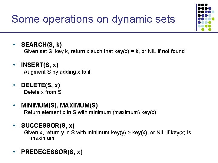
Some operations on dynamic sets • SEARCH(S, k) Given set S, key k, return x such that key(x) = k, or NIL if not found • INSERT(S, x) Augment S by adding x to it • DELETE(S, x) Delete x from S • MINIMUM(S), MAXIMUM(S) Return element x in S with minimum (maximum) key(x) • SUCCESSOR(S, x) Given x, return y in S with minimum key(y) > key(x), or NIL if key(x) is maximum • PREDECESSOR(S, x)
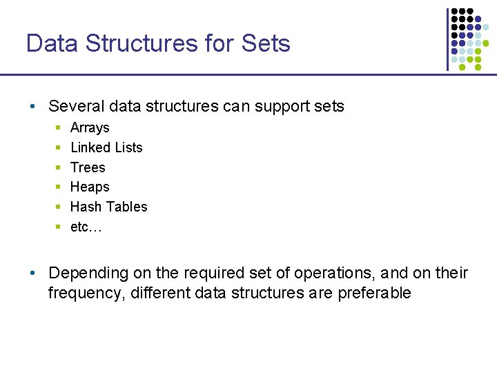
Data Structures for Sets • Several data structures can support sets § § § Arrays Linked Lists Trees Heaps Hash Tables etc… • Depending on the required set of operations, and on their frequency, different data structures are preferable
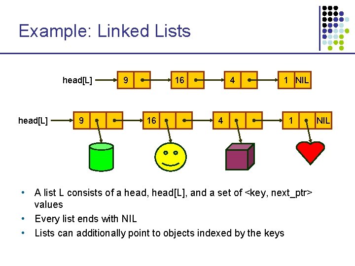
Example: Linked Lists head[L] 9 9 16 16 4 4 1 NIL 1 • A list L consists of a head, head[L], and a set of <key, next_ptr> values • Every list ends with NIL • Lists can additionally point to objects indexed by the keys NIL
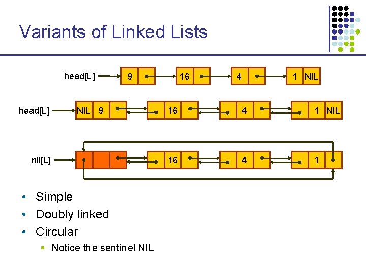
Variants of Linked Lists head[L] 9 NIL 9 nil[L] • Simple • Doubly linked • Circular § Notice the sentinel NIL 16 4 1
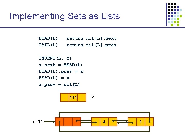
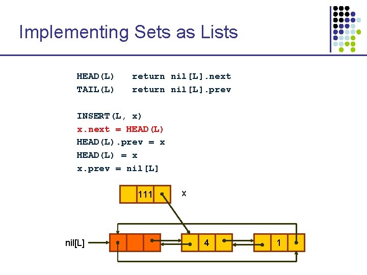
Implementing Sets as Lists HEAD(L) TAIL(L) return nil[L]. next return nil[L]. prev INSERT(L, x) x. next = HEAD(L). prev = x HEAD(L) = x x. prev = nil[L] 111 nil[L] x 4 1
Implementing Sets as Lists HEAD(L) TAIL(L) return nil[L]. next return nil[L]. prev INSERT(L, x) x. next = HEAD(L). prev = x HEAD(L) = x x. prev = nil[L] 111 nil[L] x 4 1
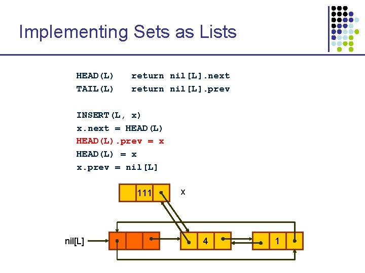
Implementing Sets as Lists HEAD(L) TAIL(L) return nil[L]. next return nil[L]. prev INSERT(L, x) x. next = HEAD(L). prev = x HEAD(L) = x x. prev = nil[L] 111 nil[L] x 4 1
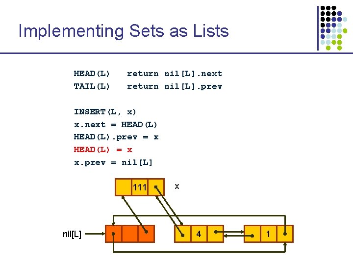
Implementing Sets as Lists HEAD(L) TAIL(L) return nil[L]. next return nil[L]. prev INSERT(L, x) x. next = HEAD(L). prev = x HEAD(L) = x x. prev = nil[L] 111 nil[L] x 4 1
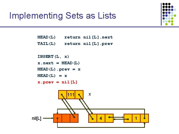
Implementing Sets as Lists HEAD(L) TAIL(L) return nil[L]. next return nil[L]. prev INSERT(L, x) x. next = HEAD(L). prev = x HEAD(L) = x x. prev = nil[L] 111 nil[L] x 4 1
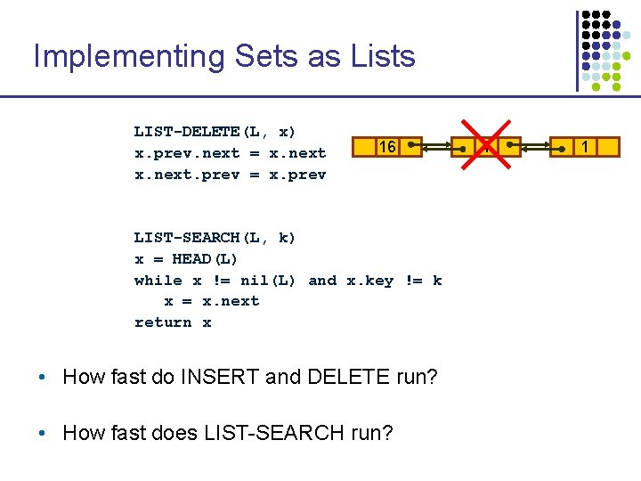
Implementing Sets as Lists LIST-DELETE(L, x) x. prev. next = x. next. prev = x. prev 16 LIST-SEARCH(L, k) x = HEAD(L) while x != nil(L) and x. key != k x = x. next return x • How fast do INSERT and DELETE run? • How fast does LIST-SEARCH run? 4 1
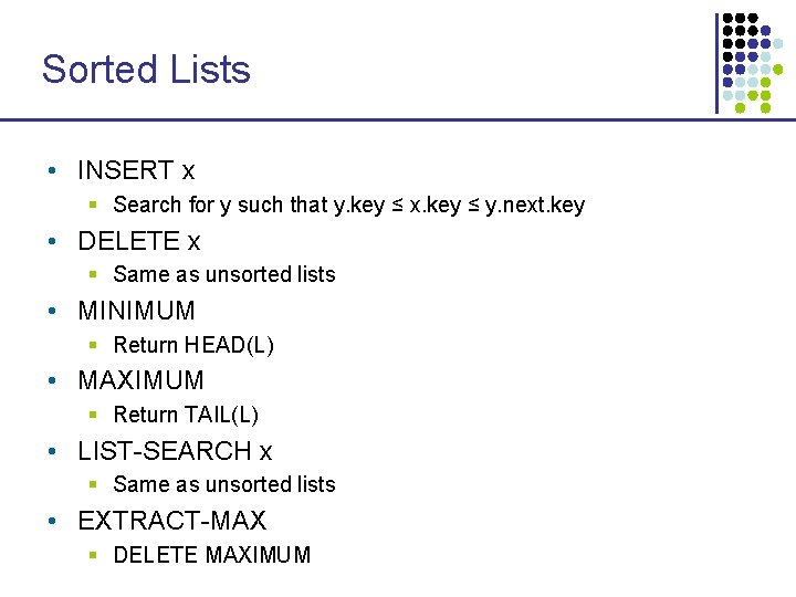
Sorted Lists • INSERT x § Search for y such that y. key ≤ x. key ≤ y. next. key • DELETE x § Same as unsorted lists • MINIMUM § Return HEAD(L) • MAXIMUM § Return TAIL(L) • LIST-SEARCH x § Same as unsorted lists • EXTRACT-MAX § DELETE MAXIMUM
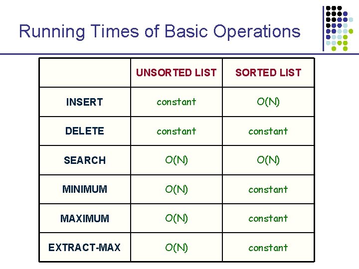
Running Times of Basic Operations UNSORTED LIST INSERT constant O(N) DELETE constant SEARCH O(N) MINIMUM O(N) constant MAXIMUM O(N) constant EXTRACT-MAX O(N) constant
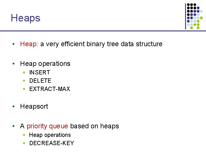
Heaps • Heap: a very efficient binary tree data structure • Heap operations § INSERT § DELETE § EXTRACT-MAX • Heapsort • A priority queue based on heaps § Heap operations § DECREASE-KEY
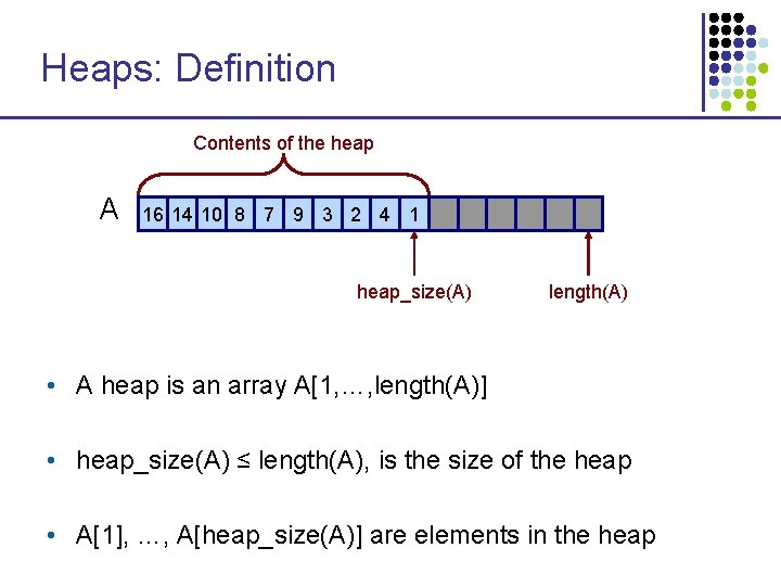
Heaps: Definition Contents of the heap A 16 14 10 8 7 9 3 2 4 1 heap_size(A) length(A) • A heap is an array A[1, …, length(A)] • heap_size(A) ≤ length(A), is the size of the heap • A[1], …, A[heap_size(A)] are elements in the heap
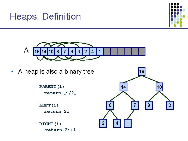
Heaps: Definition A 16 14 10 8 7 9 3 2 4 1 • A heap is also a binary tree 16 PARENT(i) return i/2 14 8 LEFT(i) return 2 i RIGHT(i) return 2 i+1 10 2 7 4 1 9 3
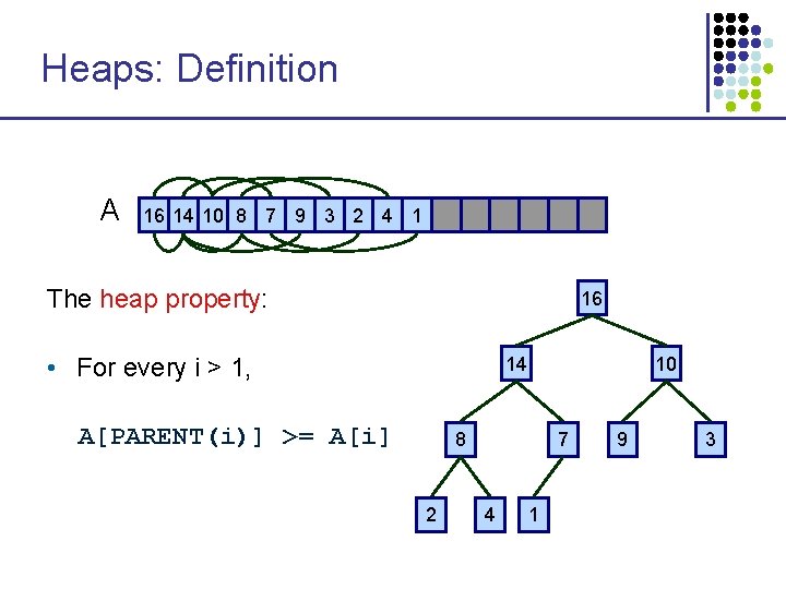
Heaps: Definition A 16 14 10 8 7 9 3 2 4 1 The heap property: 16 • For every i > 1, 14 A[PARENT(i)] >= A[i] 10 8 2 7 4 1 9 3
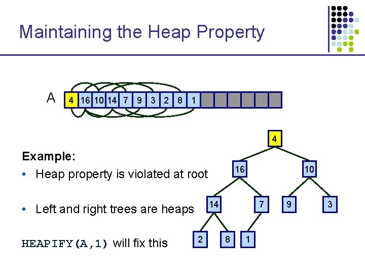
Maintaining the Heap Property A 4 16 10 14 7 9 3 2 8 1 4 Example: • Heap property is violated at root 10 14 • Left and right trees are heaps HEAPIFY(A, 1) will fix this 16 2 7 8 1 9 3
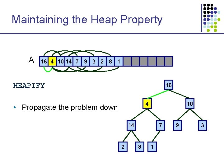
Maintaining the Heap Property A 16 4 10 14 7 9 3 2 8 1 HEAPIFY 16 4 • Propagate the problem down 10 14 2 7 8 1 9 3
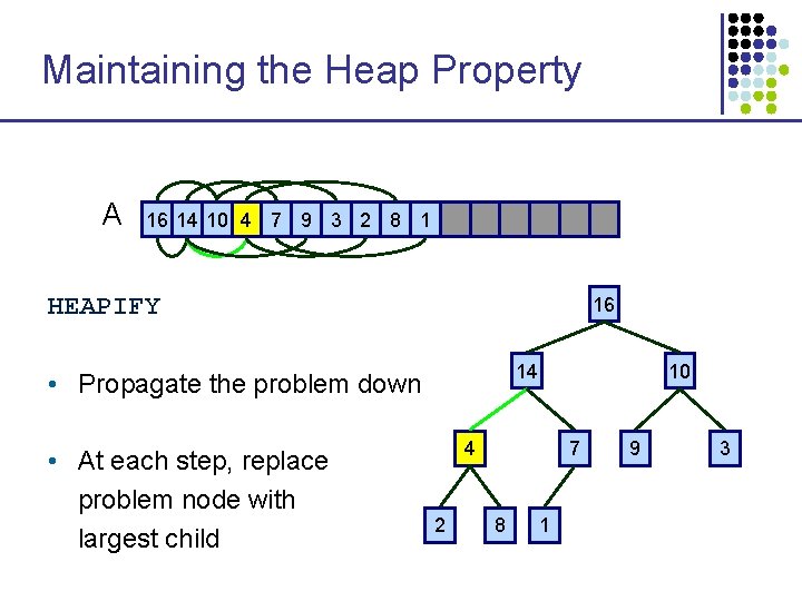
Maintaining the Heap Property A 16 14 10 4 7 9 3 2 8 1 HEAPIFY 16 14 • Propagate the problem down • At each step, replace problem node with largest child 10 4 2 7 8 1 9 3
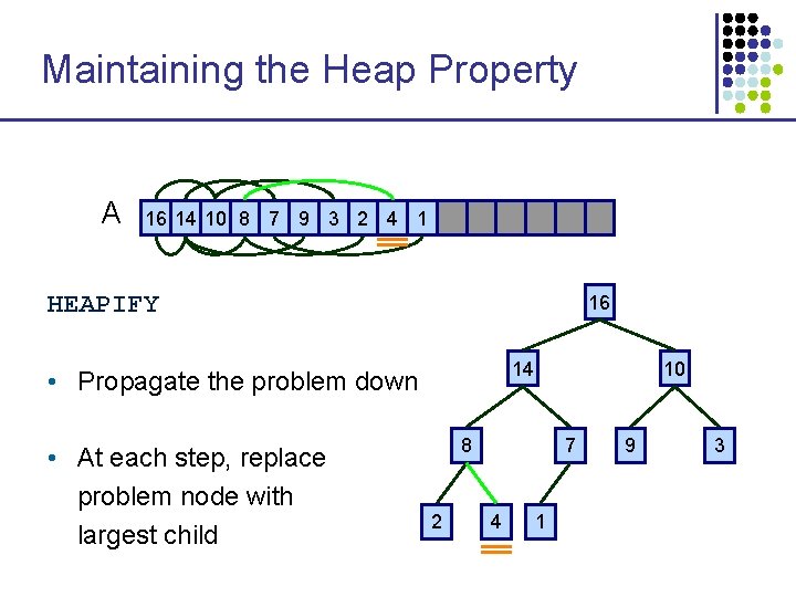
Maintaining the Heap Property A 16 14 10 8 7 9 3 2 4 1 HEAPIFY 16 14 • Propagate the problem down • At each step, replace problem node with largest child 10 8 2 7 4 1 9 3
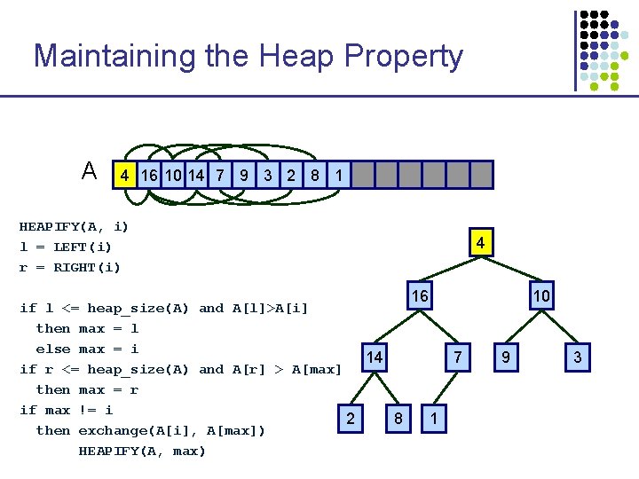
Maintaining the Heap Property A 4 16 10 14 7 9 3 2 8 1 HEAPIFY(A, i) l = LEFT(i) r = RIGHT(i) if l <= heap_size(A) and A[l]>A[i] then max = l else max = i 14 if r <= heap_size(A) and A[r] > A[max] then max = r if max != i 2 8 then exchange(A[i], A[max]) HEAPIFY(A, max) 4 16 10 7 1 9 3
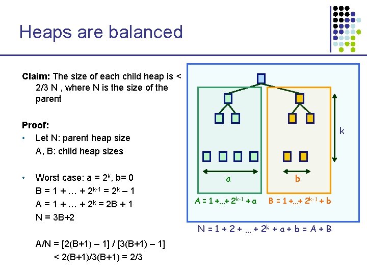
Heaps are balanced Claim: The size of each child heap is < 2/3 N , where N is the size of the parent Proof: • Let N: parent heap size A, B: child heap sizes • Worst case: a = 2 k, b= 0 B = 1 + … + 2 k-1 = 2 k – 1 A = 1 + … + 2 k = 2 B + 1 N = 3 B+2 A/N = [2(B+1) – 1] / [3(B+1) – 1] < 2(B+1)/3(B+1) = 2/3 k a A = 1 +…+ 2 k-1 + a b B = 1 +…+ 2 k-1 + b N = 1 + 2 + … + 2 k + a + b = A + B
HEAPIFY runs in time O(log n) T(n) < T(2/3 n) + (1) = (log n) by the Master Theorem [[ Case 2: T(n) = 1 T(n/ (3/2) ) + c f(n) = c; a = 1; b = 3/2; nlogba = nlog 3/21 = n 0 = 1 f(n) = (nlogba) therefore T(n) = (nlogba log n) = (log n) ]] • Alternatively, T(n) = O(h), where h is height of the heap
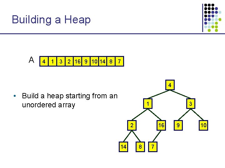
Building a Heap A 4 1 3 2 16 9 10 14 8 7 4 • Build a heap starting from an unordered array 1 3 2 14 16 8 7 9 10
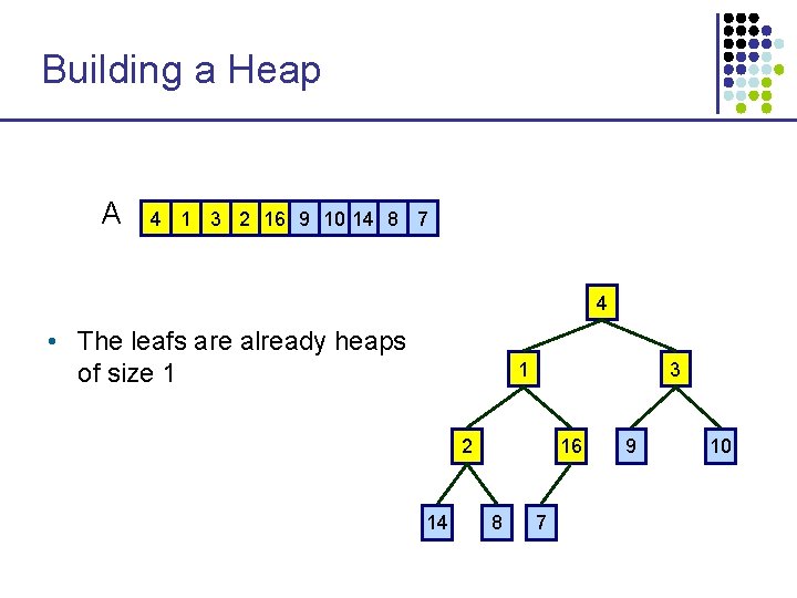
Building a Heap A 4 1 3 2 16 9 10 14 8 7 4 • The leafs are already heaps of size 1 1 3 2 14 16 8 7 9 10
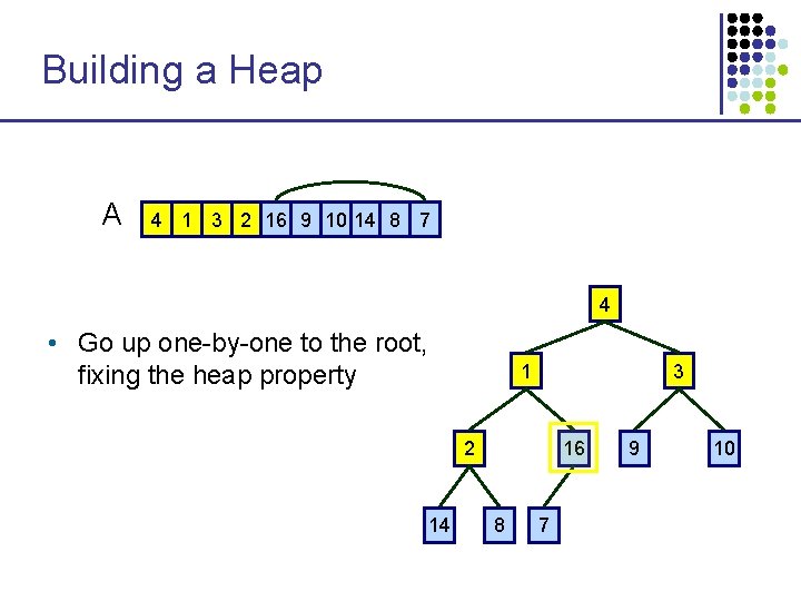
Building a Heap A 4 1 3 2 16 9 10 14 8 7 4 • Go up one-by-one to the root, fixing the heap property 1 3 2 14 16 8 7 9 10
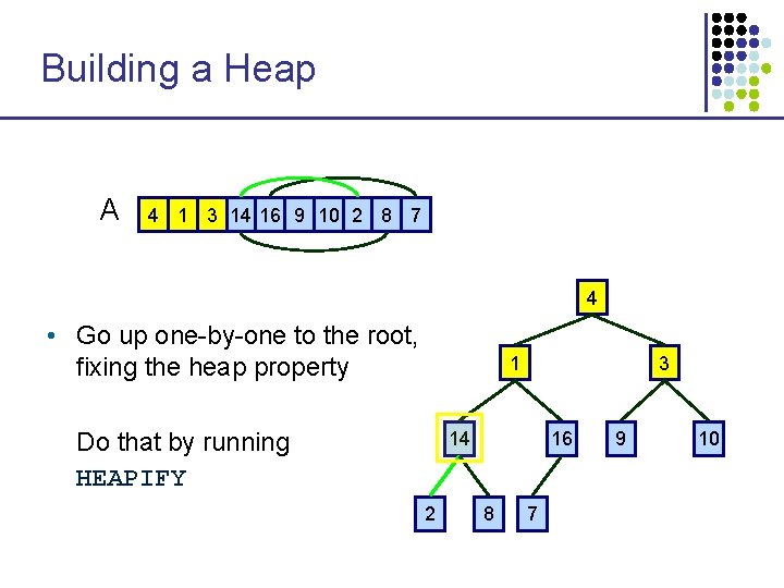
Building a Heap A 4 1 3 14 16 9 10 2 8 7 4 • Go up one-by-one to the root, fixing the heap property 1 Do that by running HEAPIFY 3 14 2 16 8 7 9 10
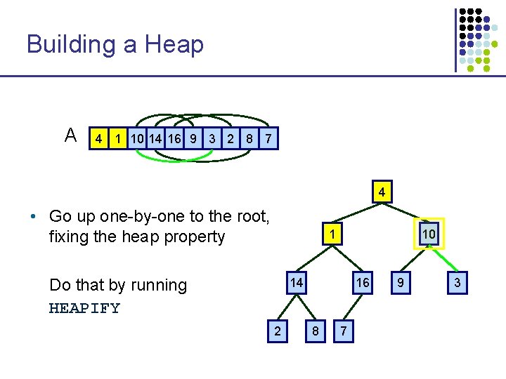
Building a Heap A 4 1 10 14 16 9 3 2 8 7 4 • Go up one-by-one to the root, fixing the heap property 1 Do that by running HEAPIFY 10 14 2 16 8 7 9 3
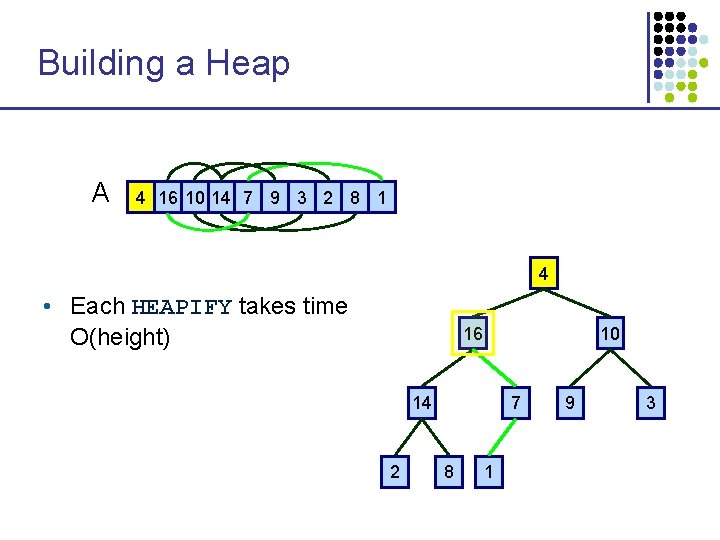
Building a Heap A 4 16 10 14 7 9 3 2 8 1 4 • Each HEAPIFY takes time O(height) 16 10 14 2 7 8 1 9 3
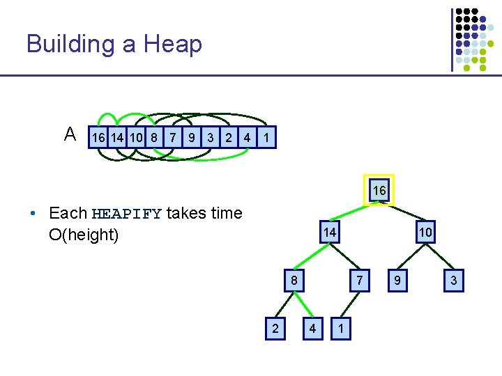
Building a Heap A 16 14 10 8 7 9 3 2 4 1 16 • Each HEAPIFY takes time O(height) 14 10 8 2 7 4 1 9 3
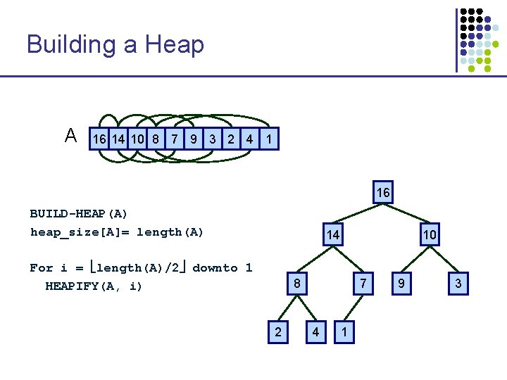
Building a Heap A 16 14 10 8 7 9 3 2 4 1 16 BUILD-HEAP(A) heap_size[A]= length(A) 14 For i = length(A)/2 downto 1 HEAPIFY(A, i) 10 8 2 7 4 1 9 3
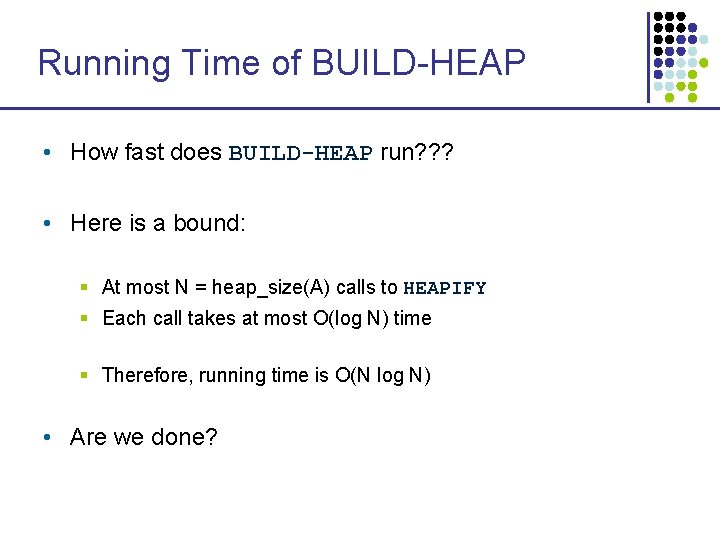
Running Time of BUILD-HEAP • How fast does BUILD-HEAP run? ? ? • Here is a bound: § At most N = heap_size(A) calls to HEAPIFY § Each call takes at most O(log N) time § Therefore, running time is O(N log N) • Are we done?
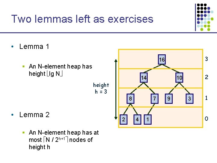
Two lemmas left as exercises • Lemma 1 3 16 § An N-element heap has height lg N 14 2 10 height h=3 8 • Lemma 2 § An N-element heap has at most N / 2 h+1 nodes of height h 2 7 4 1 9 3 1 0
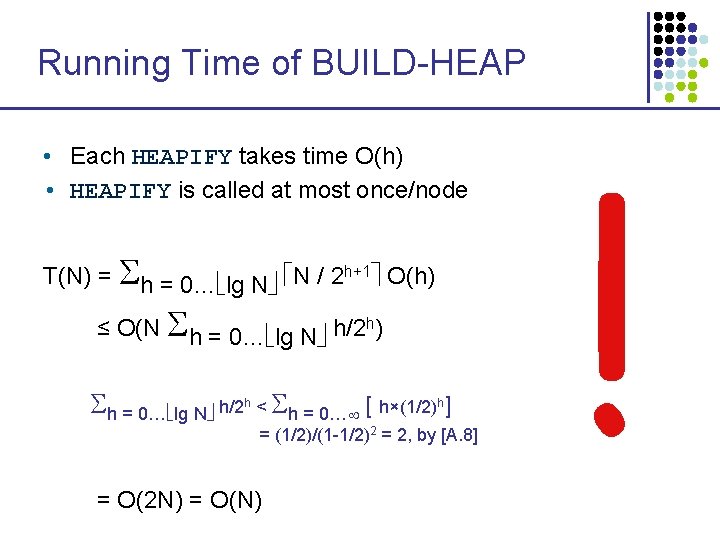
Running Time of BUILD-HEAP • Each HEAPIFY takes time O(h) • HEAPIFY is called at most once/node T(N) = h = 0… lg N N / 2 h+1 O(h) ≤ O(N h = 0… lg N h/2 h) h = 0… lg N h/2 h < h = 0… [ h×(1/2)h] = = O(2 N) = O(N) (1/2)/(1 -1/2)2 = 2, by [A. 8] !
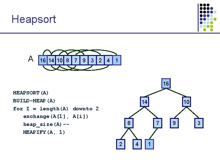
Heapsort A 16 14 10 8 7 9 3 2 4 1 16 HEAPSORT(A) BUILD-HEAP(A) for I = length(A) downto 2 exchange(A[1], A[i]) heap_size(A)-HEAPIFY(A, 1) 14 10 8 2 7 4 1 9 3
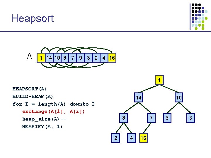
Heapsort A 16 1 14 10 8 7 9 3 2 4 16 1 HEAPSORT(A) BUILD-HEAP(A) for I = length(A) downto 2 exchange(A[1], A[i]) heap_size(A)-HEAPIFY(A, 1) 14 8 2 10 7 4 16 1 9 3
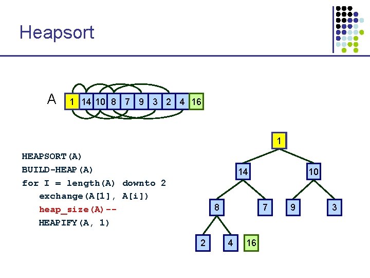
Heapsort A 16 1 14 10 8 7 9 3 2 4 16 1 HEAPSORT(A) BUILD-HEAP(A) for I = length(A) downto 2 exchange(A[1], A[i]) heap_size(A)-HEAPIFY(A, 1) 14 8 2 10 7 4 16 1 9 3
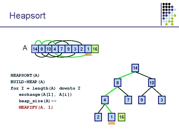
Heapsort A 14 8 10 4 7 9 3 2 1 16 1 14 HEAPSORT(A) BUILD-HEAP(A) for I = length(A) downto 2 exchange(A[1], A[i]) heap_size(A)-HEAPIFY(A, 1) 8 10 4 2 7 1 16 1 9 3
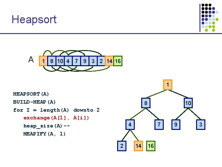
Heapsort A 1 8 10 4 7 9 3 2 14 16 1 1 HEAPSORT(A) BUILD-HEAP(A) for I = length(A) downto 2 exchange(A[1], A[i]) heap_size(A)-HEAPIFY(A, 1) 8 10 4 2 7 14 16 1 9 3
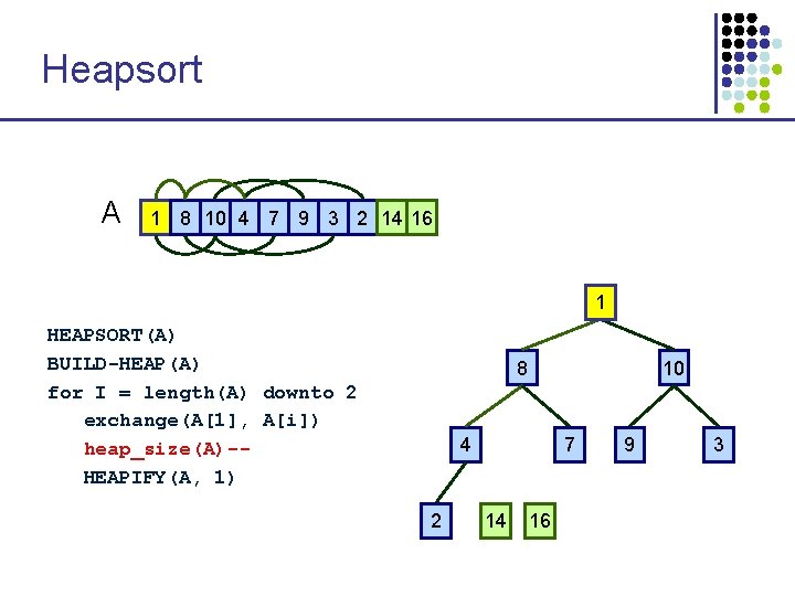
Heapsort A 1 8 10 4 7 9 3 2 14 16 1 1 HEAPSORT(A) BUILD-HEAP(A) for I = length(A) downto 2 exchange(A[1], A[i]) heap_size(A)-HEAPIFY(A, 1) 8 10 4 2 7 14 16 1 9 3
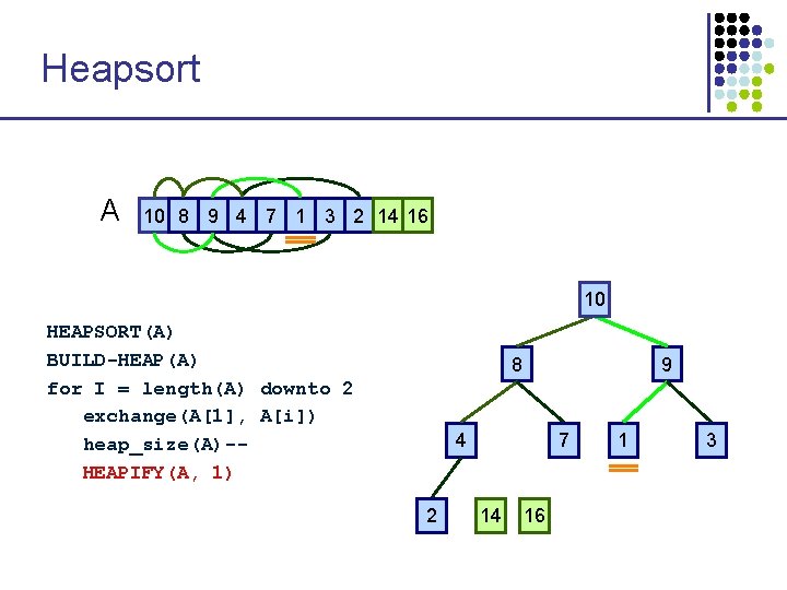
Heapsort A 10 8 9 4 7 1 3 2 14 16 1 10 HEAPSORT(A) BUILD-HEAP(A) for I = length(A) downto 2 exchange(A[1], A[i]) heap_size(A)-HEAPIFY(A, 1) 8 9 4 2 7 14 16 1 1 3
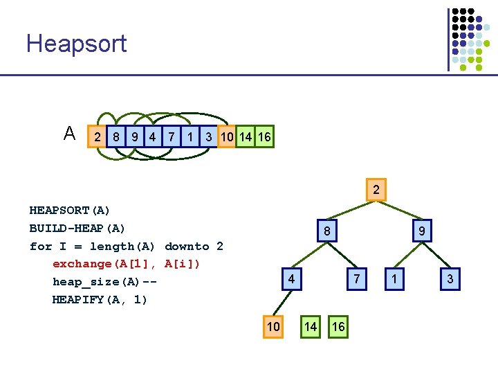
Heapsort A 2 8 9 4 7 1 3 10 14 16 1 2 HEAPSORT(A) BUILD-HEAP(A) for I = length(A) downto 2 exchange(A[1], A[i]) heap_size(A)-HEAPIFY(A, 1) 8 9 4 10 7 14 16 1 1 3
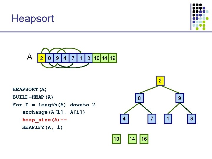
Heapsort A 2 8 9 4 7 1 3 10 14 16 1 2 HEAPSORT(A) BUILD-HEAP(A) for I = length(A) downto 2 exchange(A[1], A[i]) heap_size(A)-HEAPIFY(A, 1) 8 9 4 10 7 14 16 1 1 3
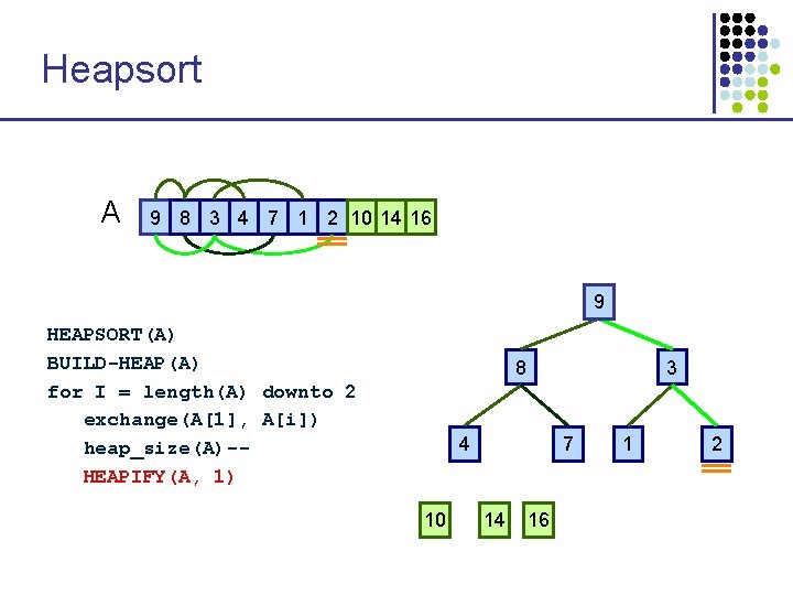
Heapsort A 9 8 3 4 7 1 2 10 14 16 1 9 HEAPSORT(A) BUILD-HEAP(A) for I = length(A) downto 2 exchange(A[1], A[i]) heap_size(A)-HEAPIFY(A, 1) 8 3 4 10 7 14 16 1 1 2
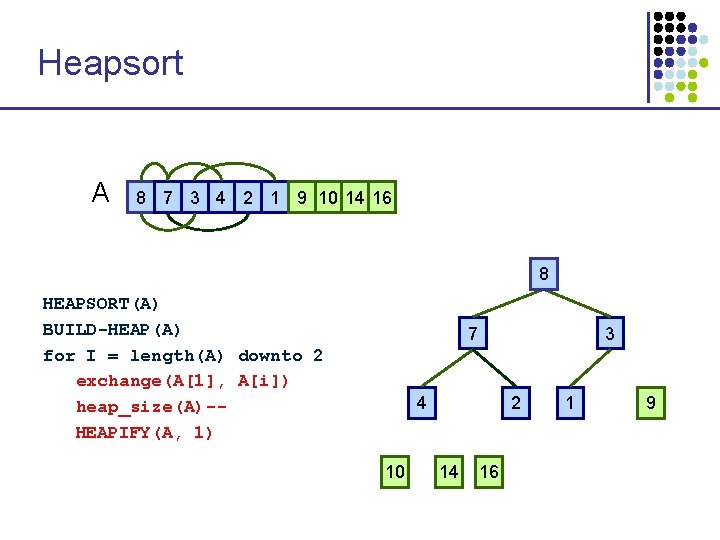
Heapsort A 8 7 3 4 2 1 9 10 14 16 1 8 HEAPSORT(A) BUILD-HEAP(A) for I = length(A) downto 2 exchange(A[1], A[i]) heap_size(A)-HEAPIFY(A, 1) 7 3 4 10 2 14 16 1 1 9
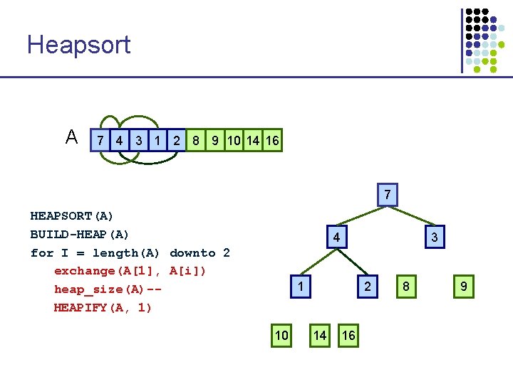
Heapsort A 7 4 3 1 2 8 9 10 14 16 1 7 HEAPSORT(A) BUILD-HEAP(A) for I = length(A) downto 2 exchange(A[1], A[i]) heap_size(A)-HEAPIFY(A, 1) 4 3 1 10 2 14 16 1 8 9
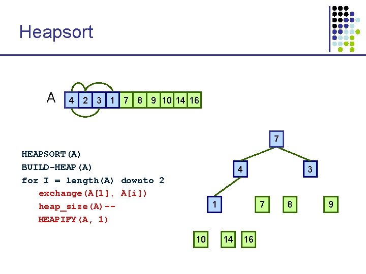
Heapsort A 4 2 3 1 7 8 9 10 14 16 1 7 HEAPSORT(A) BUILD-HEAP(A) for I = length(A) downto 2 exchange(A[1], A[i]) heap_size(A)-HEAPIFY(A, 1) 4 3 1 10 7 14 16 1 8 9
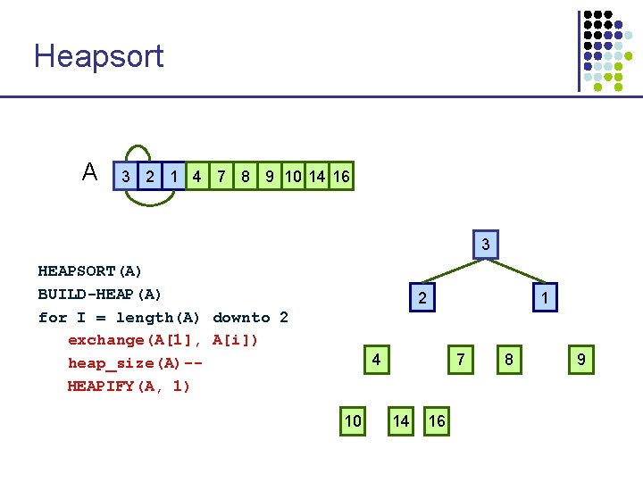
Heapsort A 3 2 1 4 7 8 9 10 14 16 1 3 HEAPSORT(A) BUILD-HEAP(A) for I = length(A) downto 2 exchange(A[1], A[i]) heap_size(A)-HEAPIFY(A, 1) 2 1 4 10 7 14 16 1 8 9
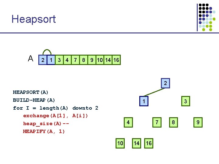
Heapsort A 2 1 3 4 7 8 9 10 14 16 1 2 HEAPSORT(A) BUILD-HEAP(A) for I = length(A) downto 2 exchange(A[1], A[i]) heap_size(A)-HEAPIFY(A, 1) 1 3 4 10 7 14 16 1 8 9
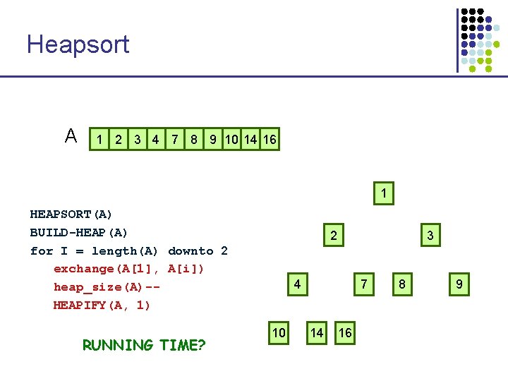
Heapsort A 1 2 3 4 7 8 9 10 14 16 1 1 HEAPSORT(A) BUILD-HEAP(A) for I = length(A) downto 2 exchange(A[1], A[i]) heap_size(A)-HEAPIFY(A, 1) RUNNING TIME? 2 3 4 10 7 14 16 1 8 9
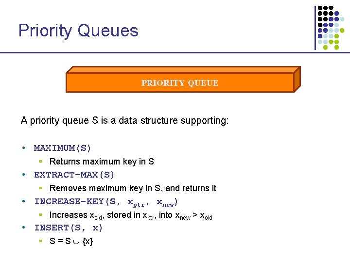
Priority Queues PRIORITY QUEUE A priority queue S is a data structure supporting: • MAXIMUM(S) § Returns maximum key in S • EXTRACT-MAX(S) § Removes maximum key in S, and returns it • INCREASE-KEY(S, xptr, xnew) § Increases xold, stored in xptr, into xnew > xold • INSERT(S, x) § S = S {x}
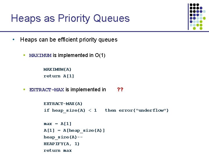
Heaps as Priority Queues • Heaps can be efficient priority queues § MAXIMUM is implemented in O(1) MAXIMUM(A) return A[1] § EXTRACT-MAX is implemented in EXTRACT-MAX(A) if heap_size(A) < 1 ? ? max = A[1] = A[heap_size(A)] heap_size(A)-HEAPIFY(A, 1) return max then error(“underflow”)
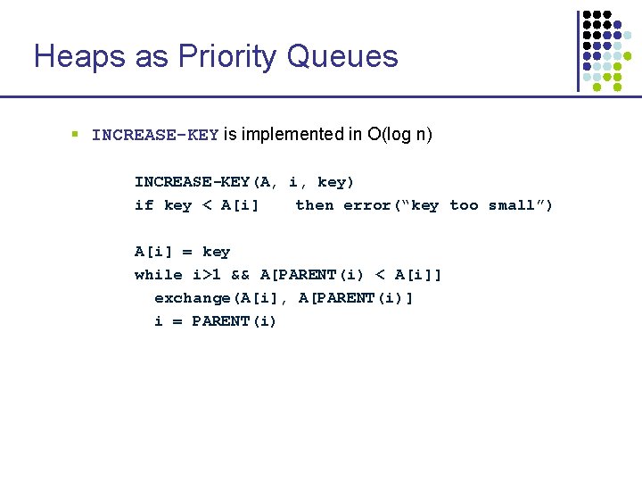
Heaps as Priority Queues § INCREASE-KEY is implemented in O(log n) INCREASE-KEY(A, i, key) if key < A[i] then error(“key too small”) A[i] = key while i>1 && A[PARENT(i) < A[i]] exchange(A[i], A[PARENT(i)] i = PARENT(i)
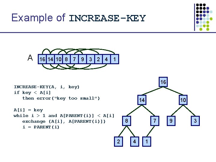
Example of INCREASE-KEY A 16 14 10 8 7 9 3 2 4 1 16 INCREASE-KEY(A, i, key) if key < A[i] then error(“key too small”) 14 A[i] = key while i > 1 and A[PARENT(i)] < A[i] exchange (A[i], A[PARENT(i)]) i = PARENT(i) 10 8 2 7 4 1 9 3
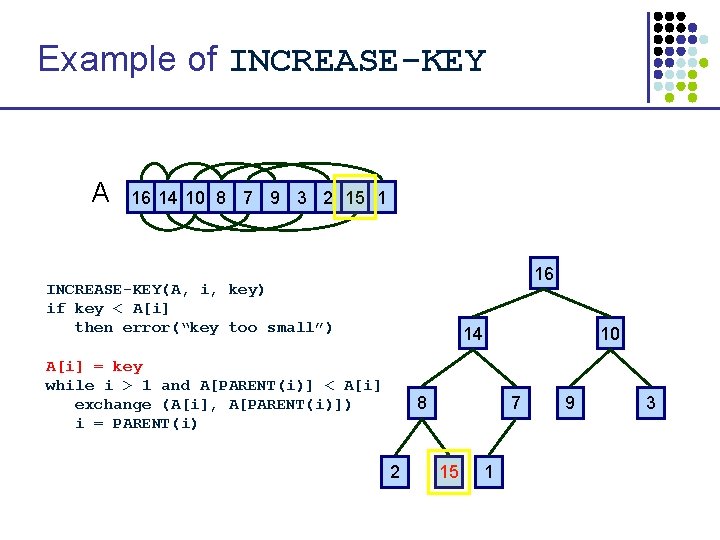
Example of INCREASE-KEY A 16 14 10 8 7 9 3 2 15 1 16 INCREASE-KEY(A, i, key) if key < A[i] then error(“key too small”) 14 A[i] = key while i > 1 and A[PARENT(i)] < A[i] exchange (A[i], A[PARENT(i)]) i = PARENT(i) 10 8 2 7 15 1 9 3
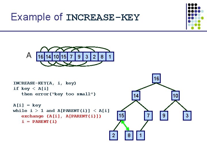
Example of INCREASE-KEY A 16 14 10 15 7 9 3 2 8 1 16 INCREASE-KEY(A, i, key) if key < A[i] then error(“key too small”) 14 A[i] = key while i > 1 and A[PARENT(i)] < A[i] exchange (A[i], A[PARENT(i)]) i = PARENT(i) 10 15 2 7 8 1 9 3
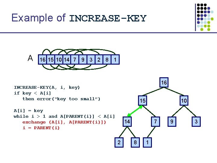
Example of INCREASE-KEY A 16 15 10 14 7 9 3 2 8 1 16 INCREASE-KEY(A, i, key) if key < A[i] then error(“key too small”) 15 A[i] = key while i > 1 and A[PARENT(i)] < A[i] exchange (A[i], A[PARENT(i)]) i = PARENT(i) 10 14 2 7 8 1 9 3
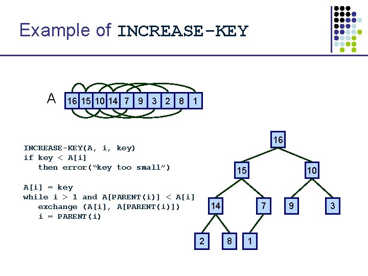
Example of INCREASE-KEY A 16 15 10 14 7 9 3 2 8 1 16 INCREASE-KEY(A, i, key) if key < A[i] then error(“key too small”) 15 A[i] = key while i > 1 and A[PARENT(i)] < A[i] exchange (A[i], A[PARENT(i)]) i = PARENT(i) 10 14 2 7 8 1 9 3
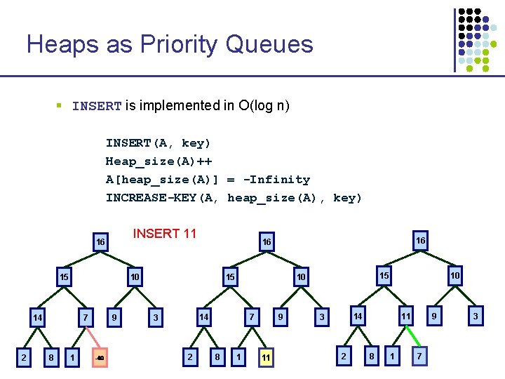
Heaps as Priority Queues § INSERT is implemented in O(log n) INSERT(A, key) Heap_size(A)++ A[heap_size(A)] = -Infinity INCREASE-KEY(A, heap_size(A), key) INSERT 11 16 15 2 7 8 15 10 14 1 9 - 16 16 14 3 2 7 8 15 10 1 9 11 10 14 3 2 11 8 1 9 7 3
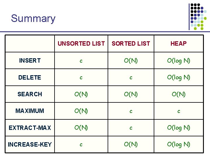
Summary UNSORTED LIST HEAP INSERT c O(N) O(log N) DELETE c c O(log N) SEARCH O(N) MAXIMUM O(N) c c EXTRACT-MAX O(N) c O(log N) INCREASE-KEY c O(N) O(log N)
- Slides: 62