Data Structures Chapter 7 Sorting 7 1 Sorting
![Heap Sort (1) Phase 1: Construct a max heap. [1 26 ] [2 5 Heap Sort (1) Phase 1: Construct a max heap. [1 26 ] [2 5](https://slidetodoc.com/presentation_image_h/11db954aaa85205f333354e3f428e601/image-27.jpg)
![Heap Sort (2) [1 26 ] Step 4 [2 61 ] 48 [4 [5 Heap Sort (2) [1 26 ] Step 4 [2 61 ] 48 [4 [5](https://slidetodoc.com/presentation_image_h/11db954aaa85205f333354e3f428e601/image-28.jpg)
![Radix Sort基數排序: Pass 1 (nondecreasing) a[1] 179 a[2] 208 a[3] 306 a[4] 93 a[5] Radix Sort基數排序: Pass 1 (nondecreasing) a[1] 179 a[2] 208 a[3] 306 a[4] 93 a[5]](https://slidetodoc.com/presentation_image_h/11db954aaa85205f333354e3f428e601/image-32.jpg)
![Radix Sort: Pass 2 a[1] 271 e[0] a[2] 93 a[3] 33 a[4] 984 a[5] Radix Sort: Pass 2 a[1] 271 e[0] a[2] 93 a[3] 33 a[4] 984 a[5]](https://slidetodoc.com/presentation_image_h/11db954aaa85205f333354e3f428e601/image-33.jpg)
![Radix Sort: Pass 3 a[1] 306 a[2] 208 a[3] 9 a[4] 33 a[5] 55 Radix Sort: Pass 3 a[1] 306 a[2] 208 a[3] 9 a[4] 33 a[5] 55](https://slidetodoc.com/presentation_image_h/11db954aaa85205f333354e3f428e601/image-34.jpg)
![Construction of Huffman Tree 5 3 2 (a) [2, 3, 5, 7, 9, 13] Construction of Huffman Tree 5 3 2 (a) [2, 3, 5, 7, 9, 13]](https://slidetodoc.com/presentation_image_h/11db954aaa85205f333354e3f428e601/image-53.jpg)
- Slides: 57

Data Structures Chapter 7: Sorting 7 -1

Sorting (1) • List: a collection of records – Each record has one or more fields. – Key: used to distinguish among the records. Record 1 Record 2 Record 3 Key 4 2 1 Other fields DDD BBB AAA Key 1 2 3 Other fields AAA BBB CCC Record 4 Record 5 5 3 EEE CCC 4 5 DDD EEE original list sorted list 7 -2

Sorting (2) Original pointer list File Record 1 Record 2 4 DDD Record 3 Record 4 2 BBB 1 AAA 5 EEE 3 CCC Record 5 Sorted pointer list • It is easier to search a particular element after sorting. (e. g. binary search) • best sorting algorithm with comparisons: 7 -3 O(nlogn)

Sequential Search • Applied to an array or a linked list. • Data are not sorted. • Example: 9 5 6 8 7 2 – search 6: successful search – search 4: unsuccessful search • # of comparisons for a successful search on record key i is i. • Time complexity – successful search: (n+1)/2 comparisons = O(n) – unsuccessful search: n comparisons = O(n) 7 -4

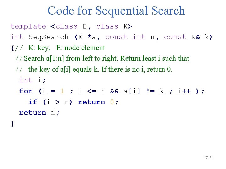
Code for Sequential Search template <class E, class K> int Seq. Search (E *a, const int n, const K& k) {// K: key, E: node element //Search a[1: n] from left to right. Return least i such that // the key of a[i] equals k. If there is no i, return 0. int i; for (i = 1 ; i <= n && a[i] != k ; i++ ); if (i > n) return 0; return i; } 7 -5

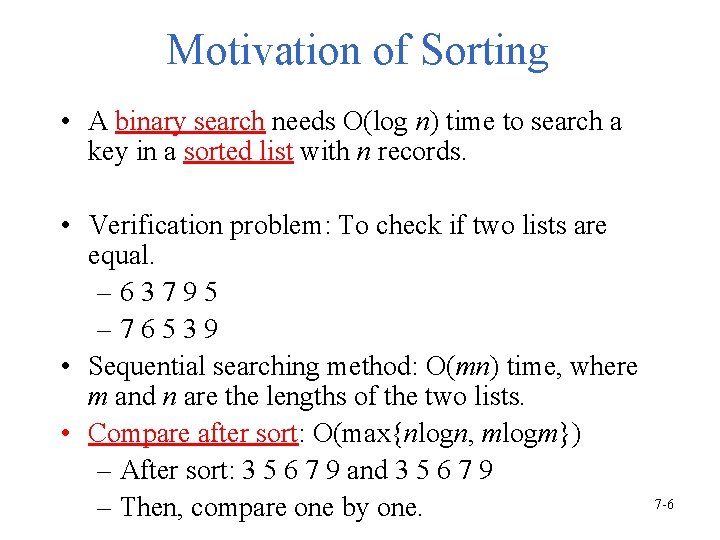
Motivation of Sorting • A binary search needs O(log n) time to search a key in a sorted list with n records. • Verification problem: To check if two lists are equal. – 63795 – 76539 • Sequential searching method: O(mn) time, where m and n are the lengths of the two lists. • Compare after sort: O(max{nlogn, mlogm}) – After sort: 3 5 6 7 9 and 3 5 6 7 9 – Then, compare one by one. 7 -6

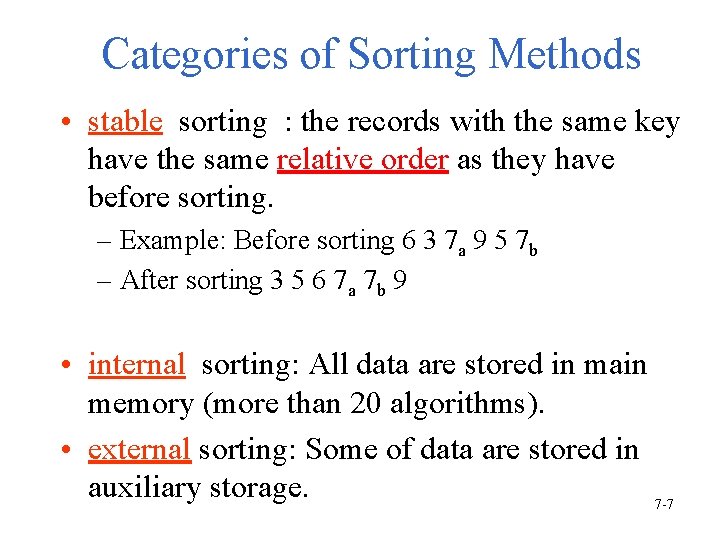
Categories of Sorting Methods • stable sorting : the records with the same key have the same relative order as they have before sorting. – Example: Before sorting 6 3 7 a 9 5 7 b – After sorting 3 5 6 7 a 7 b 9 • internal sorting: All data are stored in main memory (more than 20 algorithms). • external sorting: Some of data are stored in auxiliary storage. 7 -7

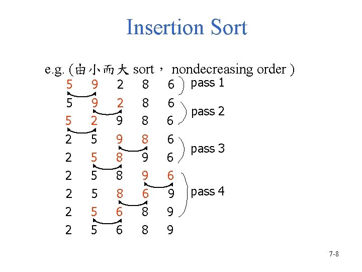
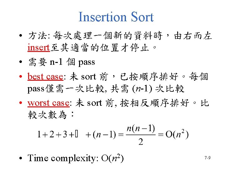
Insertion Sort e. g. (由小而大 sort, nondecreasing order ) 5 9 2 8 6 pass 1 5 5 9 2 2 9 8 8 6 6 pass 2 2 5 9 8 6 2 5 8 9 6 2 5 8 6 9 2 5 6 8 9 pass 3 pass 4 7 -8


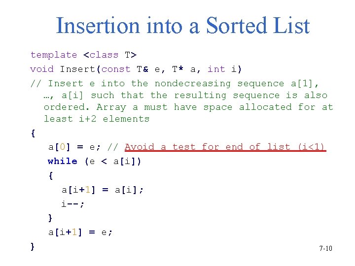
Insertion into a Sorted List template <class T> void Insert(const T& e, T* a, int i) // Insert e into the nondecreasing sequence a[1], …, a[i] such that the resulting sequence is also ordered. Array a must have space allocated for at least i+2 elements { a[0] = e; // Avoid a test for end of list (i<1) while (e < a[i]) { a[i+1] = a[i]; i--; } a[i+1] = e; } 7 -10

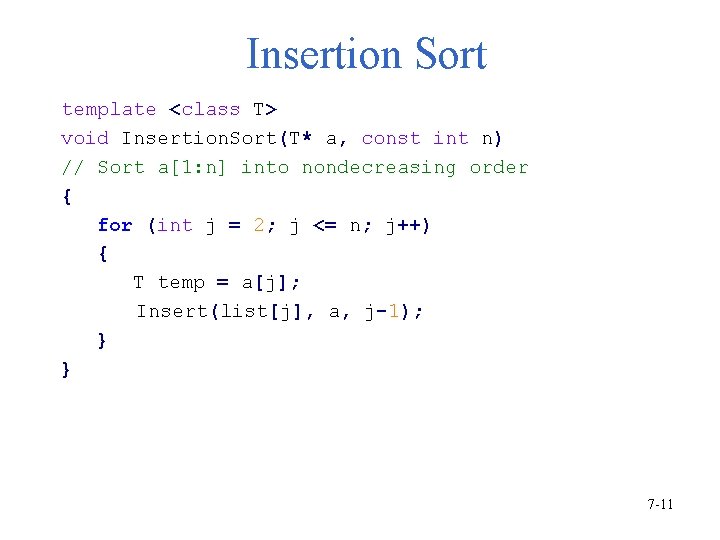
Insertion Sort template <class T> void Insertion. Sort(T* a, const int n) // Sort a[1: n] into nondecreasing order { for (int j = 2; j <= n; j++) { T temp = a[j]; Insert(list[j], a, j-1); } } 7 -11

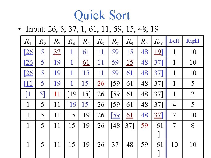
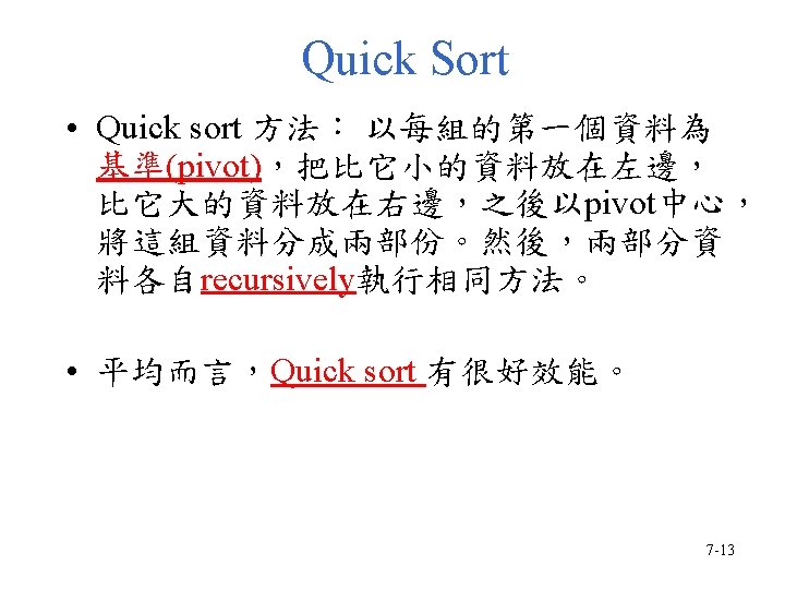
Quick Sort • Input: 26, 5, 37, 1, 61, 11, 59, 15, 48, 19 R 1 R 2 [26 5 [11 5 [1 5] 1 5 R 3 R 4 R 5 37 1 61 19 1 15] 11 [19 15] R 6 R 7 R 8 11 59 15 11 59 61 26 [59 61 R 9 48 48 48 R 10 Left 19] 1 37] 1 37] 4 Right 10 10 10 5 2 5 1 1 5 5 11 11 15 15 19 19 26 [59 61 48 37] 26 [48 37] 59 [61 ] 7 7 10 8 1 5 11 15 19 26 10 10 37 48 59 [61 ]


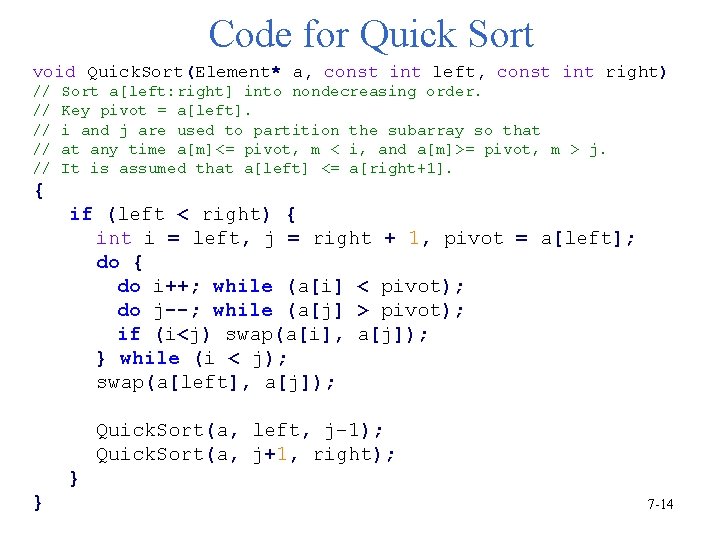
Code for Quick Sort void Quick. Sort(Element* a, const int left, const int right) // // // Sort a[left: right] into nondecreasing order. Key pivot = a[left]. i and j are used to partition the subarray so that at any time a[m]<= pivot, m < i, and a[m]>= pivot, m > j. It is assumed that a[left] <= a[right+1]. { if (left < right) { int i = left, j = right + 1, pivot = a[left]; do { do i++; while (a[i] < pivot); do j--; while (a[j] > pivot); if (i<j) swap(a[i], a[j]); } while (i < j); swap(a[left], a[j]); Quick. Sort(a, left, j– 1); Quick. Sort(a, j+1, right); } } 7 -14

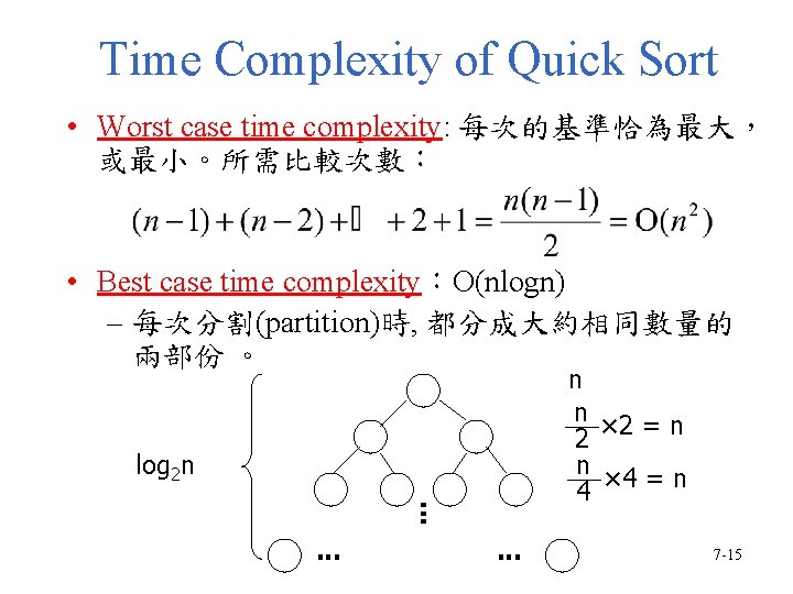
Time Complexity of Quick Sort • Worst case time complexity: 每次的基準恰為最大, 或最小。所需比較次數: • Best case time complexity:O(nlogn) – 每次分割(partition)時, 都分成大約相同數量的 兩部份 。 n n × 2 = n 2 n × 4 = n 4 log 2 n. . 7 -15

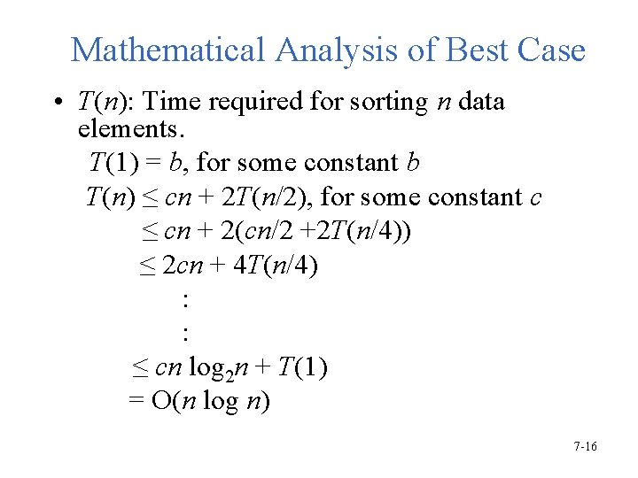
Mathematical Analysis of Best Case • T(n): Time required for sorting n data elements. T(1) = b, for some constant b T(n) ≤ cn + 2 T(n/2), for some constant c ≤ cn + 2(cn/2 +2 T(n/4)) ≤ 2 cn + 4 T(n/4) : : ≤ cn log 2 n + T(1) = O(n log n) 7 -16

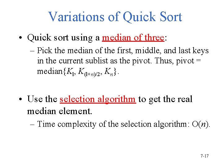
Variations of Quick Sort • Quick sort using a median of three: – Pick the median of the first, middle, and last keys in the current sublist as the pivot. Thus, pivot = median{Kl, K(l+n)/2, Kn}. • Use the selection algorithm to get the real median element. – Time complexity of the selection algorithm: O(n). 7 -17

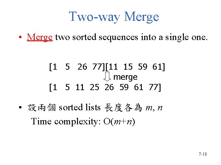
Two-way Merge • Merge two sorted sequences into a single one. [1 5 26 77][11 15 59 61] merge [1 5 11 25 26 59 61 77] • 設兩個 sorted lists 長度各為 m, n Time complexity: O(m+n) 7 -18

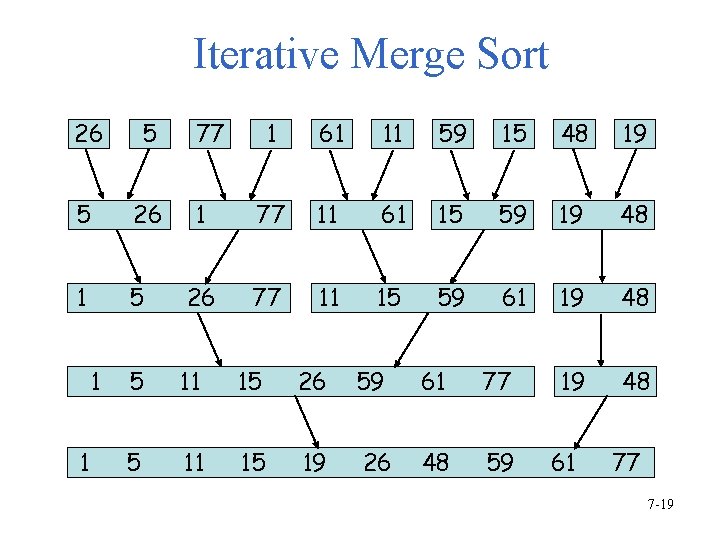
Iterative Merge Sort 26 5 5 26 1 5 1 1 77 1 61 11 59 15 48 19 1 77 11 61 15 59 19 48 26 77 11 15 59 61 19 48 5 11 15 26 59 61 77 5 11 15 19 26 48 59 61 77 7 -19

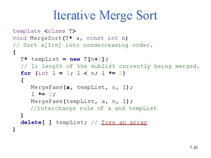
Iterative Merge Sort template <class T> void Merge. Sort(T* a, const int n) // Sort a[1: n] into nondecreasing order. { T* temp. List = new T[n+1]; // l: length of the sublist currently being merged. for (int l = 1; l < n; l *= 2) { Merge. Pass(a, temp. List, n, l); l *= 2; Merge. Pass(temp. List, a, n, l); //interchange role of a and temp. List } delete[ ] temp. List; // free an array } 7 -20

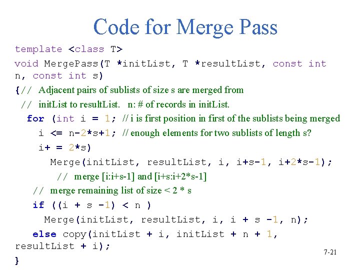
Code for Merge Pass template <class T> void Merge. Pass(T *init. List, T *result. List, const int n, const int s) {// Adjacent pairs of sublists of size s are merged from // init. List to result. List. n: # of records in init. List. for (int i = 1; // i is first position in first of the sublists being merged i <= n-2*s+1; // enough elements for two sublists of length s? i+ = 2*s) Merge(init. List, result. List, i, i+s-1, i+2*s-1); // merge [i: i+s-1] and [i+s: i+2*s-1] // merge remaining list of size < 2 * s if ((i + s -1) < n ) Merge(init. List, result. List, i, i + s -1, n); else copy(init. List + i, init. List + n + 1, result. List + i); 7 -21 }

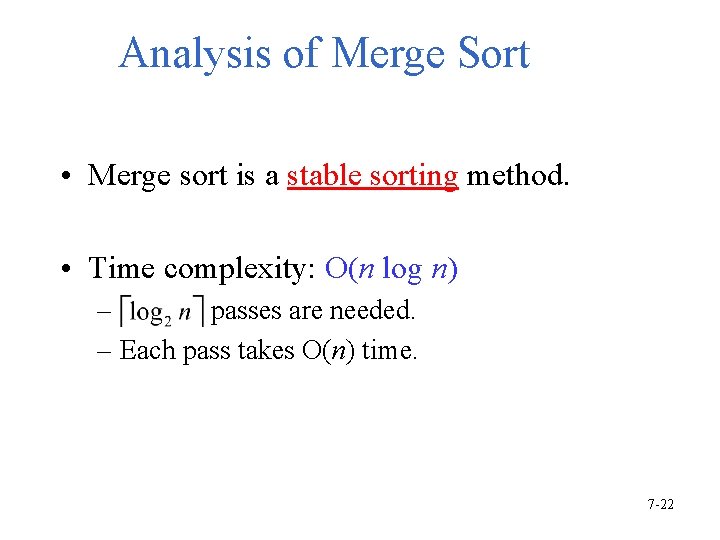
Analysis of Merge Sort • Merge sort is a stable sorting method. • Time complexity: O(n log n) – passes are needed. – Each pass takes O(n) time. 7 -22

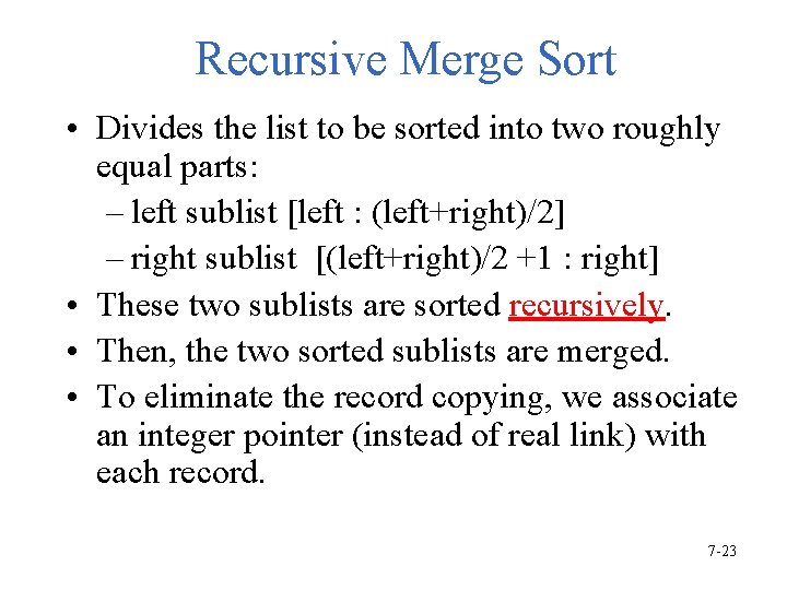
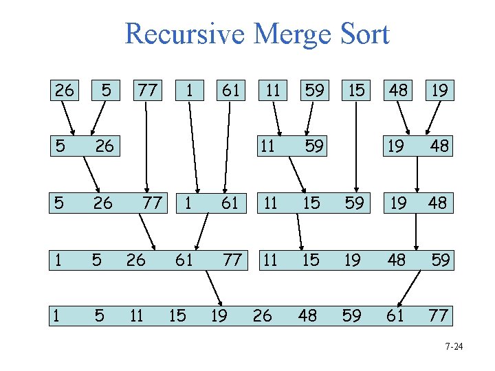
Recursive Merge Sort • Divides the list to be sorted into two roughly equal parts: – left sublist [left : (left+right)/2] – right sublist [(left+right)/2 +1 : right] • These two sublists are sorted recursively. • Then, the two sorted sublists are merged. • To eliminate the record copying, we associate an integer pointer (instead of real link) with each record. 7 -23

Recursive Merge Sort 26 5 77 5 26 1 5 11 77 1 61 11 59 15 48 19 19 48 1 61 11 15 59 19 48 61 77 11 15 19 48 59 26 48 59 61 77 15 19 7 -24

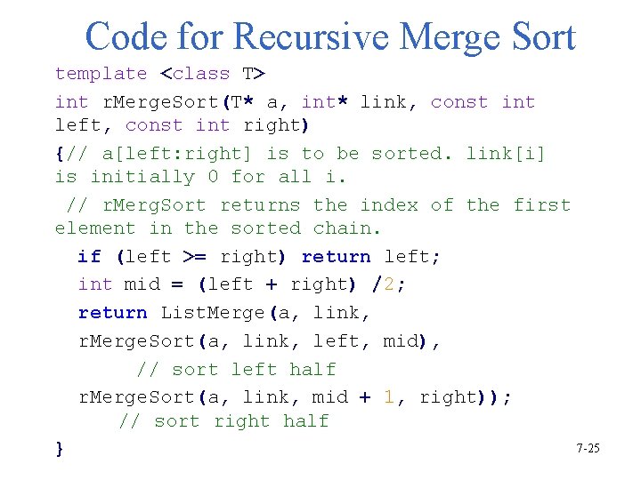
Code for Recursive Merge Sort template <class T> int r. Merge. Sort(T* a, int* link, const int left, const int right) {// a[left: right] is to be sorted. link[i] is initially 0 for all i. // r. Merg. Sort returns the index of the first element in the sorted chain. if (left >= right) return left; int mid = (left + right) /2; return List. Merge(a, link, r. Merge. Sort(a, link, left, mid), // sort left half r. Merge. Sort(a, link, mid + 1, right)); // sort right half 7 -25 }

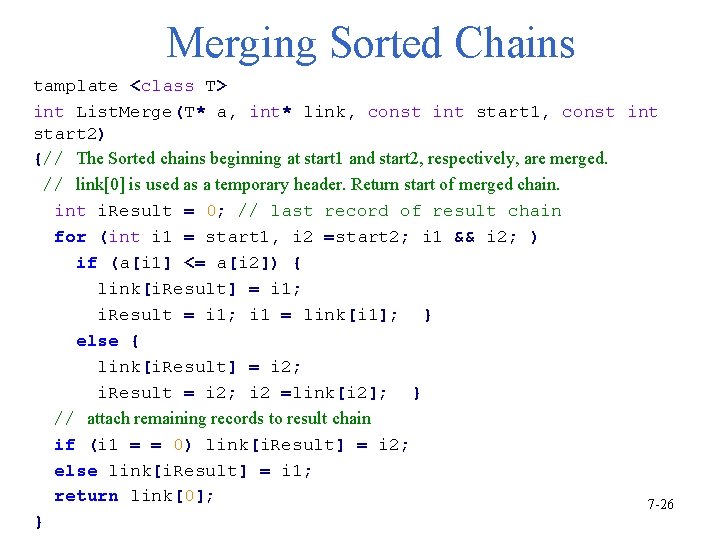
Merging Sorted Chains tamplate <class T> int List. Merge(T* a, int* link, const int start 1, const int start 2) {// The Sorted chains beginning at start 1 and start 2, respectively, are merged. // link[0] is used as a temporary header. Return start of merged chain. int i. Result = 0; // last record of result chain for (int i 1 = start 1, i 2 =start 2; i 1 && i 2; ) if (a[i 1] <= a[i 2]) { link[i. Result] = i 1; i. Result = i 1; i 1 = link[i 1]; } else { link[i. Result] = i 2; i. Result = i 2; i 2 =link[i 2]; } // attach remaining records to result chain if (i 1 = = 0) link[i. Result] = i 2; else link[i. Result] = i 1; return link[0]; 7 -26 }
![Heap Sort 1 Phase 1 Construct a max heap 1 26 2 5 Heap Sort (1) Phase 1: Construct a max heap. [1 26 ] [2 5](https://slidetodoc.com/presentation_image_h/11db954aaa85205f333354e3f428e601/image-27.jpg)
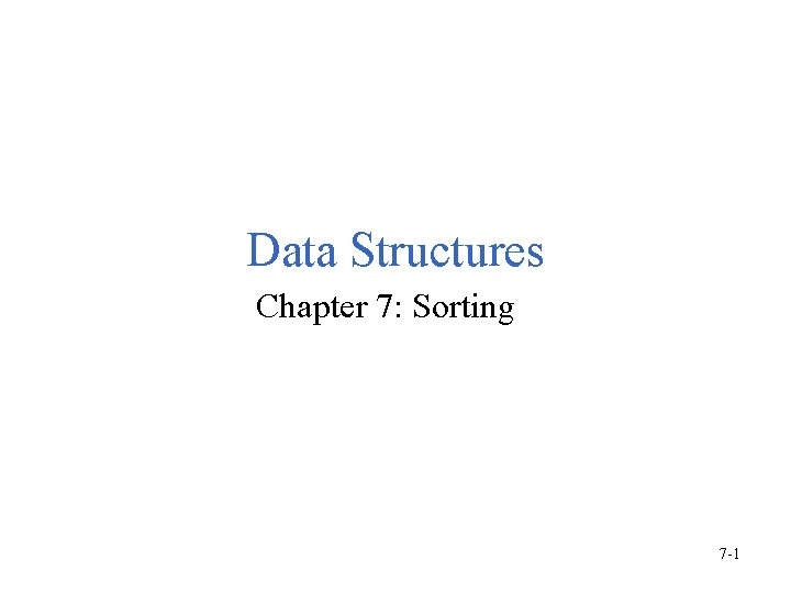
Heap Sort (1) Phase 1: Construct a max heap. [1 26 ] [2 5 ] [4 ] 1 [5 61 ] 15 48 19 [8 ] [9 ] [10 ] [3 77 ] [2 5 Step]2 11 59 [6 ] [7] (a) Input array 48 [4 ] [1 26 ] Step 1 [5 61 ] 15 1 19 [8 ] [9 ] [10 ] [3 77 ] 11 59 [6 ] [7] (b) After Adjusting 61, 1 7 -27
![Heap Sort 2 1 26 Step 4 2 61 48 4 5 Heap Sort (2) [1 26 ] Step 4 [2 61 ] 48 [4 [5](https://slidetodoc.com/presentation_image_h/11db954aaa85205f333354e3f428e601/image-28.jpg)
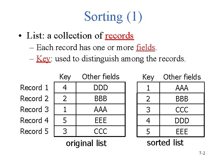
Heap Sort (2) [1 26 ] Step 4 [2 61 ] 48 [4 [5 19 ] ] 15 1 5 [8 ] [9 ] [10 ] [1 77 ] Step 3 [3 77 ] [2 61 ] 11 59 [6 ] [7] (c) After Adjusting 77, 5 48 [4 [5 19 ] ] 15 1 5 [8 ] [9 ] [10] [3 59 ] 11 26 [6 ] [7] (d) Max heap after constructing 7 -28

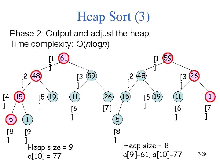
Heap Sort (3) Phase 2: Output and adjust the heap. Time complexity: O(nlogn) [2 48 ] [4 15 ] [1 61 ] [5 19 ] 5 1 [8 ] [9 ] [2 48 ] [3 59 ] 11 26 [6 ] [7] Heap size = 9 a[10] = 77 15 5 [8 ] [1 59 ] [5 19 ] [3 26 ] 11 1 [6 ] [7 ] Heap size = 8 a[9]=61, a[10]=77 7 -29

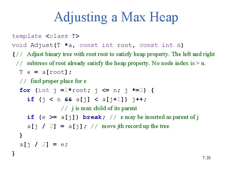
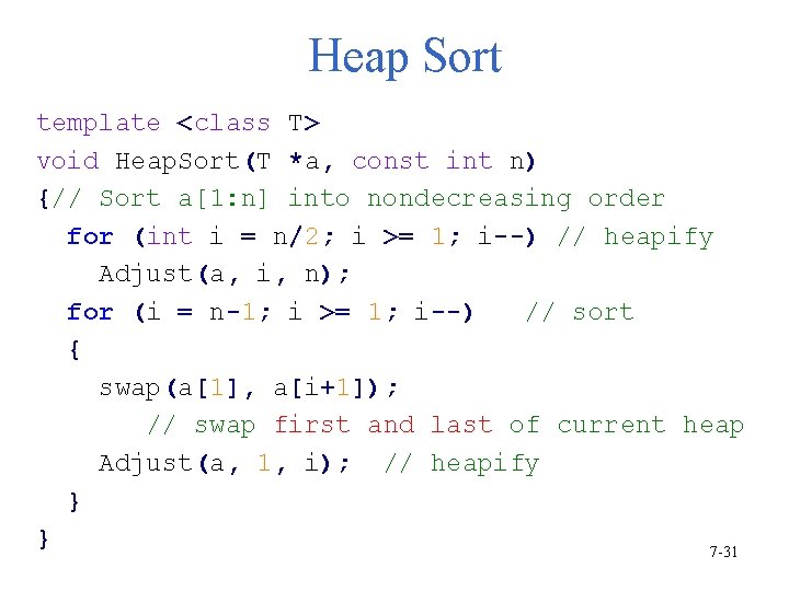
Adjusting a Max Heap template <class T> void Adjust(T *a, const int root, const int n) {// Adjust binary tree with root to satisfy heap property. The left and right // subtrees of root already satisfy the heap property. No node index is > n. T e = a[root]; // find proper place for (int j =2*root; j <= n; j *=2) { if (j < n && a[j] < a[j+1]) j++; // j is max child of its parent if (e >= a[j]) break; // e may be inserted as parent of j a[j / 2] = a[j]; // move jth record up the tree } a[j / 2] = e; } 7 -30

Heap Sort template <class T> void Heap. Sort(T *a, const int n) {// Sort a[1: n] into nondecreasing order for (int i = n/2; i >= 1; i--) // heapify Adjust(a, i, n); for (i = n-1; i >= 1; i--) // sort { swap(a[1], a[i+1]); // swap first and last of current heap Adjust(a, 1, i); // heapify } } 7 -31
![Radix Sort基數排序 Pass 1 nondecreasing a1 179 a2 208 a3 306 a4 93 a5 Radix Sort基數排序: Pass 1 (nondecreasing) a[1] 179 a[2] 208 a[3] 306 a[4] 93 a[5]](https://slidetodoc.com/presentation_image_h/11db954aaa85205f333354e3f428e601/image-32.jpg)
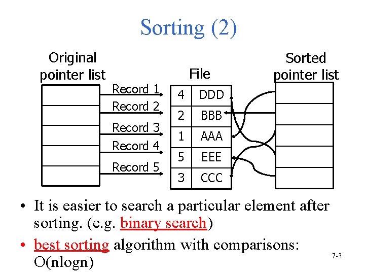
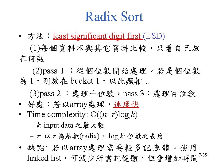
Radix Sort基數排序: Pass 1 (nondecreasing) a[1] 179 a[2] 208 a[3] 306 a[4] 93 a[5] 859 a[6] 984 a[7] 55 a[8] 9 e[0] e[1] e[2] e[3] e[4] e[5] e[6] e[7] a[9] 271 e[8] a[10] 33 e[9] 9 33 271 859 93 984 55 306 f[0] f[1] f[2] f[3] f[4] f[5] f[6] f[7] a[1] 271 a[2] 93 a[3] 33 a[4] 984 a[5] 55 a[6] 306 a[7] 208 a[8] 179 208 179 f[8] f[9] a[9] 859 a[10] 9 7 -32
![Radix Sort Pass 2 a1 271 e0 a2 93 a3 33 a4 984 a5 Radix Sort: Pass 2 a[1] 271 e[0] a[2] 93 a[3] 33 a[4] 984 a[5]](https://slidetodoc.com/presentation_image_h/11db954aaa85205f333354e3f428e601/image-33.jpg)
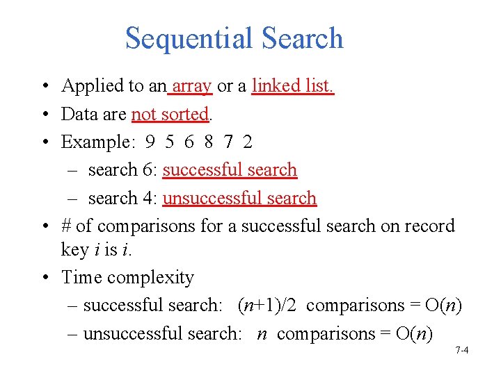
Radix Sort: Pass 2 a[1] 271 e[0] a[2] 93 a[3] 33 a[4] 984 a[5] 55 a[6] 306 a[7] 208 a[8] 179 a[9] 859 a[10] 9 e[1] e[2] e[3] e[4] e[5] e[6] e[7] e[8] e[9] 9 208 306 f[0] a[1] 306 33 859 179 55 271 984 93 f[9] f[1] f[2] f[3] f[4] f[5] f[6] f[7] f[8] a[2] 208 a[3] 9 a[4] 33 a[5] 55 a[6] 859 a[7] 271 a[8] 179 a[9] 984 a[10] 93 7 -33
![Radix Sort Pass 3 a1 306 a2 208 a3 9 a4 33 a5 55 Radix Sort: Pass 3 a[1] 306 a[2] 208 a[3] 9 a[4] 33 a[5] 55](https://slidetodoc.com/presentation_image_h/11db954aaa85205f333354e3f428e601/image-34.jpg)
Radix Sort: Pass 3 a[1] 306 a[2] 208 a[3] 9 a[4] 33 a[5] 55 a[6] 859 a[7] 271 a[8] 179 e[0] e[1] e[2] e[3] e[4] e[5] e[6] e[7] a[9] 984 a[10] 93 e[8] e[9] 859 984 f[9] 93 55 33 271 9 179 208 306 f[0] f[1] f[2] f[3] f[4] f[5] f[6] f[7] f[8] a[1] 9 a[2] 33 a[3] 55 a[4] 93 a[5] 179 a[6] 208 a[7] 271 a[8] 306 a[9] 859 a[10] 984 7 -34


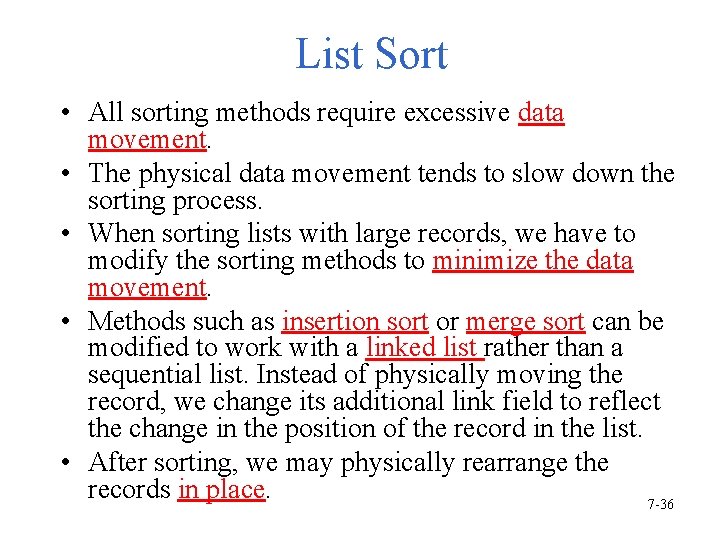
List Sort • All sorting methods require excessive data movement. • The physical data movement tends to slow down the sorting process. • When sorting lists with large records, we have to modify the sorting methods to minimize the data movement. • Methods such as insertion sort or merge sort can be modified to work with a linked list rather than a sequential list. Instead of physically moving the record, we change its additional link field to reflect the change in the position of the record in the list. • After sorting, we may physically rearrange the records in place. 7 -36

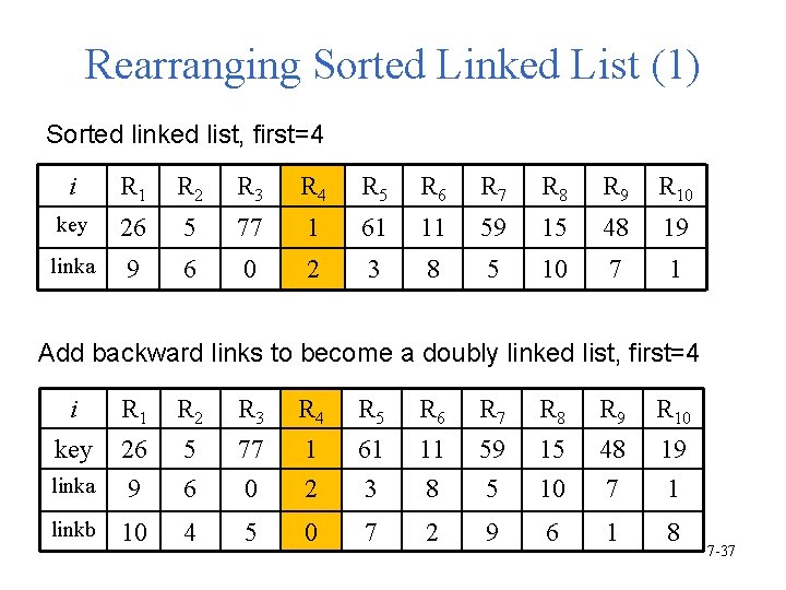
Rearranging Sorted Linked List (1) Sorted linked list, first=4 i R 1 R 2 R 3 R 4 R 5 R 6 R 7 R 8 R 9 R 10 key 26 5 77 1 61 11 59 15 48 19 linka 9 6 0 2 3 8 5 10 7 1 Add backward links to become a doubly linked list, first=4 i R 1 R 2 R 3 R 4 R 5 R 6 R 7 R 8 R 9 R 10 key 26 5 77 1 61 11 59 15 48 19 linka 9 6 0 2 3 8 5 10 7 1 linkb 10 4 5 0 7 2 9 6 1 8 7 -37

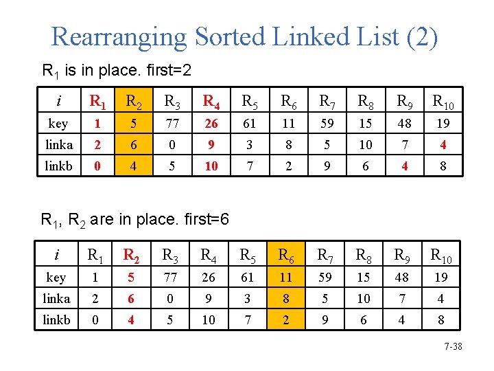
Rearranging Sorted Linked List (2) R 1 is in place. first=2 i R 1 R 2 R 3 R 4 R 5 R 6 R 7 R 8 R 9 R 10 key 1 5 77 26 61 11 59 15 48 19 linka 2 6 0 9 3 8 5 10 7 4 linkb 0 4 5 10 7 2 9 6 4 8 R 1, R 2 are in place. first=6 i R 1 R 2 R 3 R 4 R 5 R 6 R 7 R 8 R 9 R 10 key 1 5 77 26 61 11 59 15 48 19 linka 2 6 0 9 3 8 5 10 7 4 linkb 0 4 5 10 7 2 9 6 4 8 7 -38

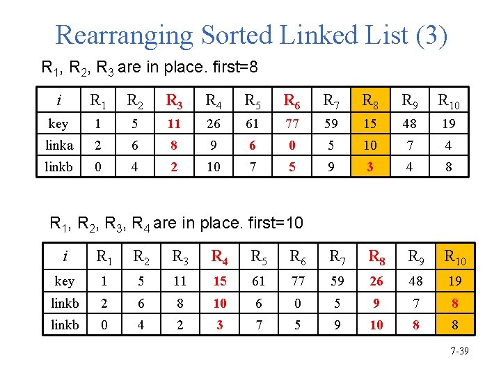
Rearranging Sorted Linked List (3) R 1, R 2, R 3 are in place. first=8 i R 1 R 2 R 3 R 4 R 5 R 6 R 7 R 8 R 9 R 10 key 1 5 11 26 61 77 59 15 48 19 linka 2 6 8 9 6 0 5 10 7 4 linkb 0 4 2 10 7 5 9 3 4 8 R 1, R 2, R 3, R 4 are in place. first=10 i R 1 R 2 R 3 R 4 R 5 R 6 R 7 R 8 R 9 R 10 key 1 5 11 15 61 77 59 26 48 19 linkb 2 6 8 10 6 0 5 9 7 8 linkb 0 4 2 3 7 5 9 10 8 8 7 -39

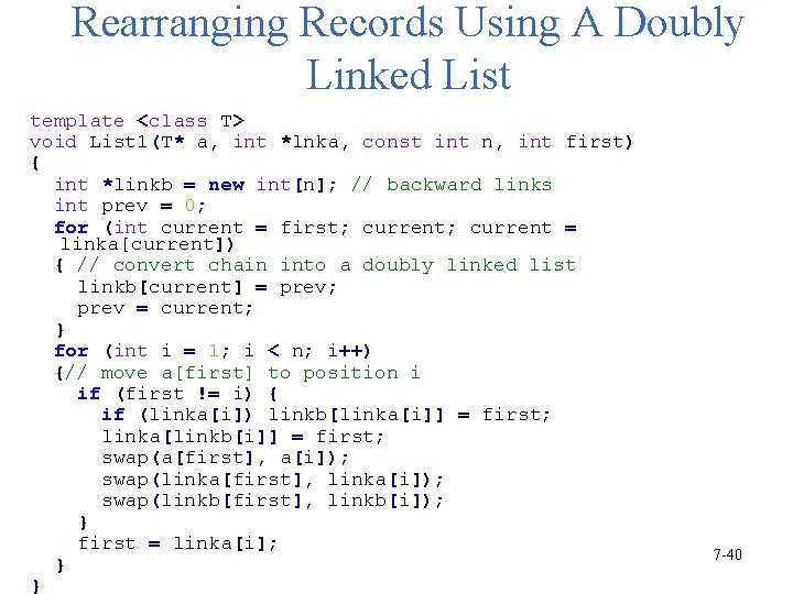
Rearranging Records Using A Doubly Linked List template <class T> void List 1(T* a, int *lnka, const int n, int first) { int *linkb = new int[n]; // backward links int prev = 0; for (int current = first; current = linka[current]) { // convert chain into a doubly linked list linkb[current] = prev; prev = current; } for (int i = 1; i < n; i++) {// move a[first] to position i if (first != i) { if (linka[i]) linkb[linka[i]] = first; linka[linkb[i]] = first; swap(a[first], a[i]); swap(linka[first], linka[i]); swap(linkb[first], linkb[i]); } first = linka[i]; } } 7 -40

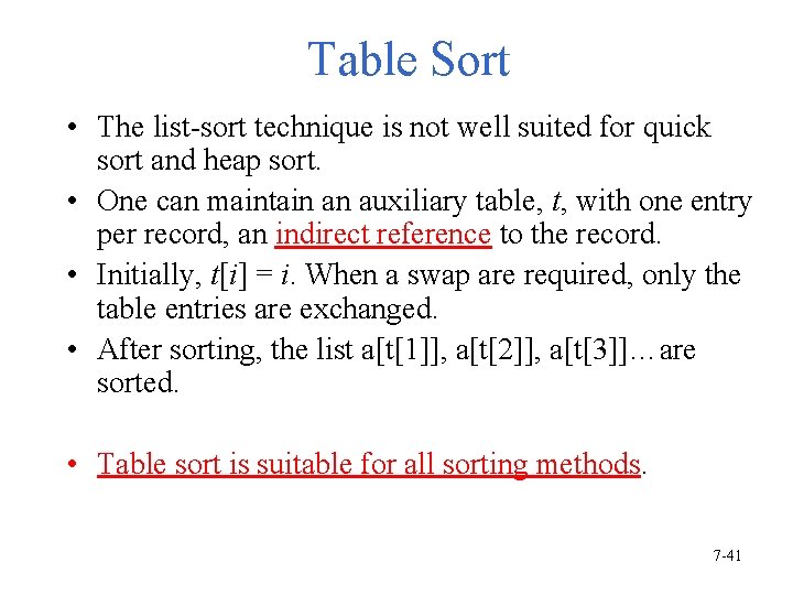
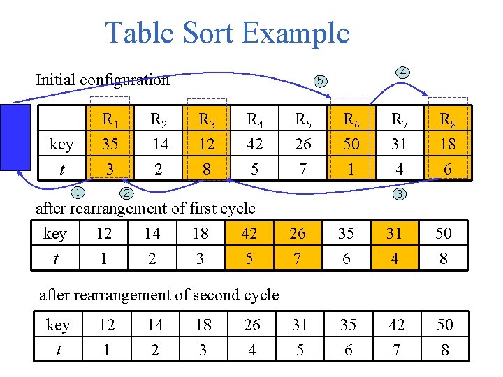
Table Sort • The list-sort technique is not well suited for quick sort and heap sort. • One can maintain an auxiliary table, t, with one entry per record, an indirect reference to the record. • Initially, t[i] = i. When a swap are required, only the table entries are exchanged. • After sorting, the list a[t[1]], a[t[2]], a[t[3]]…are sorted. • Table sort is suitable for all sorting methods. 7 -41

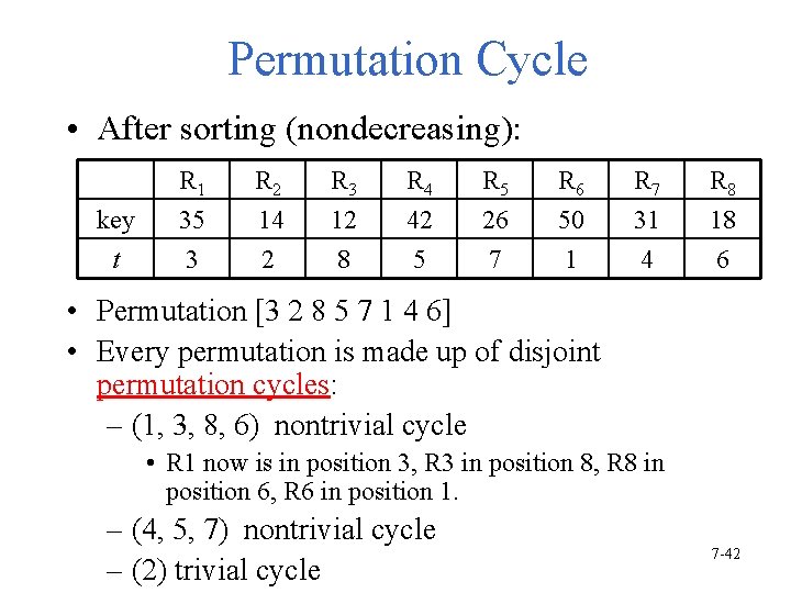
Permutation Cycle • After sorting (nondecreasing): R 1 R 2 R 3 R 4 R 5 R 6 R 7 R 8 key 35 14 12 42 26 50 31 18 t 3 2 8 5 7 1 4 6 • Permutation [3 2 8 5 7 1 4 6] • Every permutation is made up of disjoint permutation cycles: – (1, 3, 8, 6) nontrivial cycle • R 1 now is in position 3, R 3 in position 8, R 8 in position 6, R 6 in position 1. – (4, 5, 7) nontrivial cycle – (2) trivial cycle 7 -42

Table Sort Example Initial configuration 4 5 R 1 R 2 R 3 R 4 R 5 R 6 R 7 R 8 key 35 14 12 42 26 50 31 18 t 3 2 8 5 7 1 4 6 1 2 3 after rearrangement of first cycle key t 12 1 14 2 18 3 42 5 26 7 35 6 31 4 50 8 31 5 35 6 42 7 50 8 after rearrangement of second cycle key t 12 1 14 2 18 3 26 4

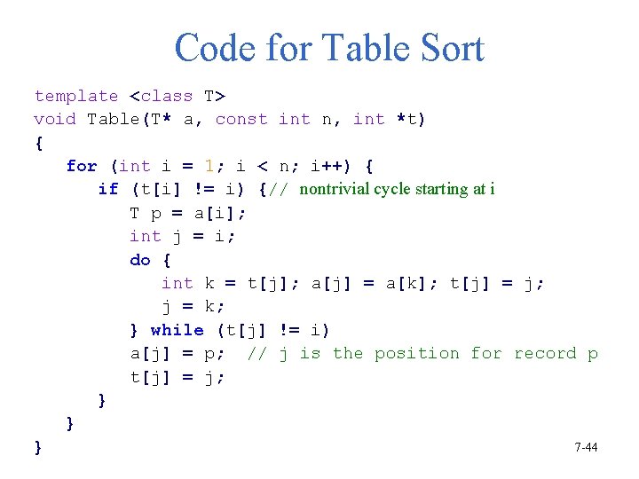
Code for Table Sort template <class T> void Table(T* a, const int n, int *t) { for (int i = 1; i < n; i++) { if (t[i] != i) {// nontrivial cycle starting at i T p = a[i]; int j = i; do { int k = t[j]; a[j] = a[k]; t[j] = j; j = k; } while (t[j] != i) a[j] = p; // j is the position for record p t[j] = j; } } 7 -44 }

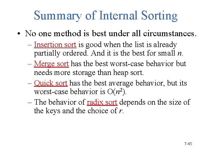
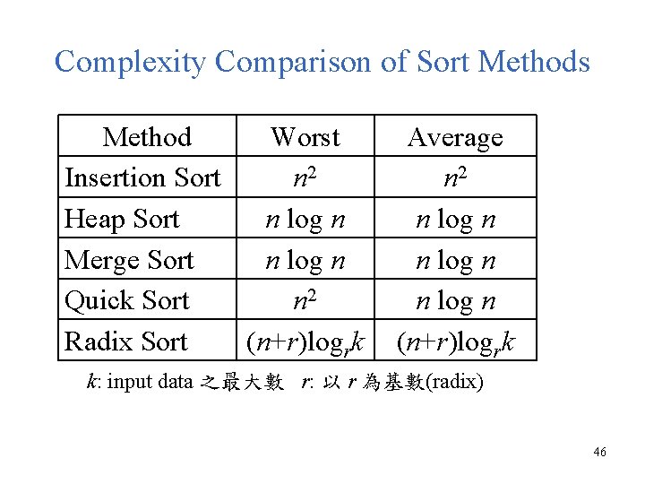
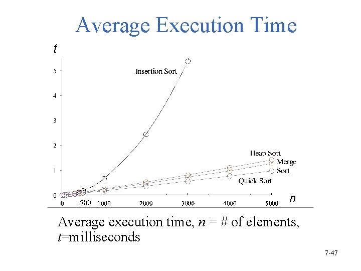
Summary of Internal Sorting • No one method is best under all circumstances. – Insertion sort is good when the list is already partially ordered. And it is the best for small n. – Merge sort has the best worst-case behavior but needs more storage than heap sort. – Quick sort has the best average behavior, but its worst-case behavior is O(n 2). – The behavior of radix sort depends on the size of the keys and the choice of r. 7 -45

Complexity Comparison of Sort Methods Method Worst Insertion Sort n 2 Heap Sort n log n Merge Sort n log n Quick Sort n 2 Radix Sort (n+r)logrk Average n 2 n log n (n+r)logrk k: input data 之最大數 r: 以 r 為基數(radix) 46

Average Execution Time t n Average execution time, n = # of elements, t=milliseconds 7 -47

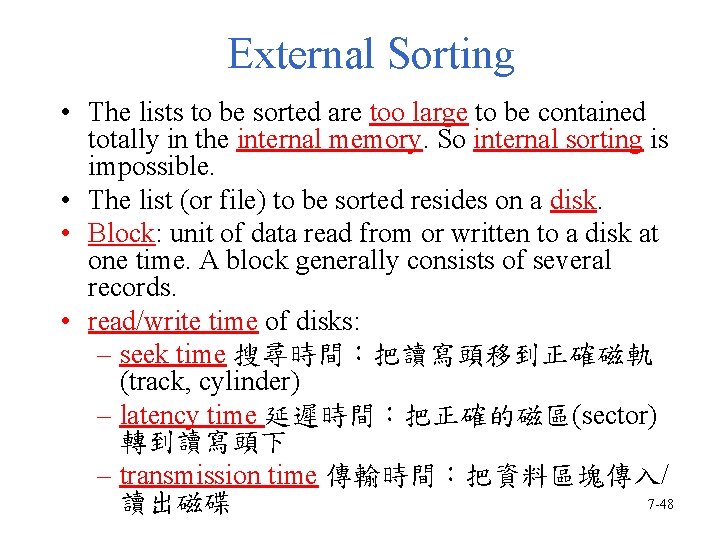
External Sorting • The lists to be sorted are too large to be contained totally in the internal memory. So internal sorting is impossible. • The list (or file) to be sorted resides on a disk. • Block: unit of data read from or written to a disk at one time. A block generally consists of several records. • read/write time of disks: – seek time 搜尋時間:把讀寫頭移到正確磁軌 (track, cylinder) – latency time 延遲時間:把正確的磁區(sector) 轉到讀寫頭下 – transmission time 傳輸時間:把資料區塊傳入/ 7 -48 讀出磁碟

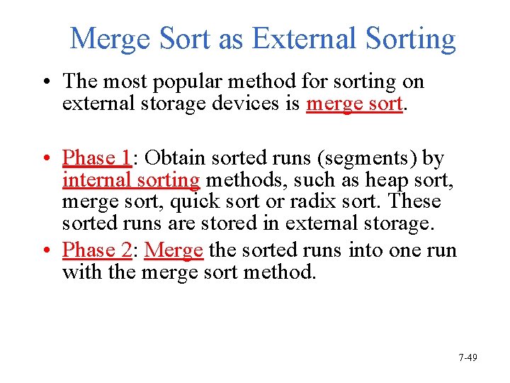
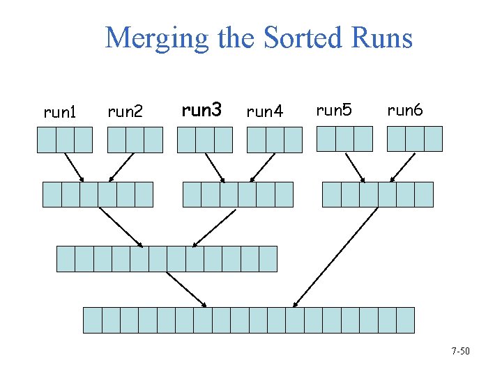
Merge Sort as External Sorting • The most popular method for sorting on external storage devices is merge sort. • Phase 1: Obtain sorted runs (segments) by internal sorting methods, such as heap sort, merge sort, quick sort or radix sort. These sorted runs are stored in external storage. • Phase 2: Merge the sorted runs into one run with the merge sort method. 7 -49

Merging the Sorted Runs run 1 run 2 run 3 run 4 run 5 run 6 7 -50

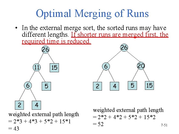
Optimal Merging of Runs • In the external merge sort, the sorted runs may have different lengths. If shorter runs are merged first, the required time is reduced. 26 26 11 6 5 2 4 weighted external path length = 2*3 + 4*3 + 5*2 + 15*1 = 43 20 6 15 2 4 5 15 weighted external path length = 2*2 + 4*2 + 5*2 + 15*2 = 52 7 -51

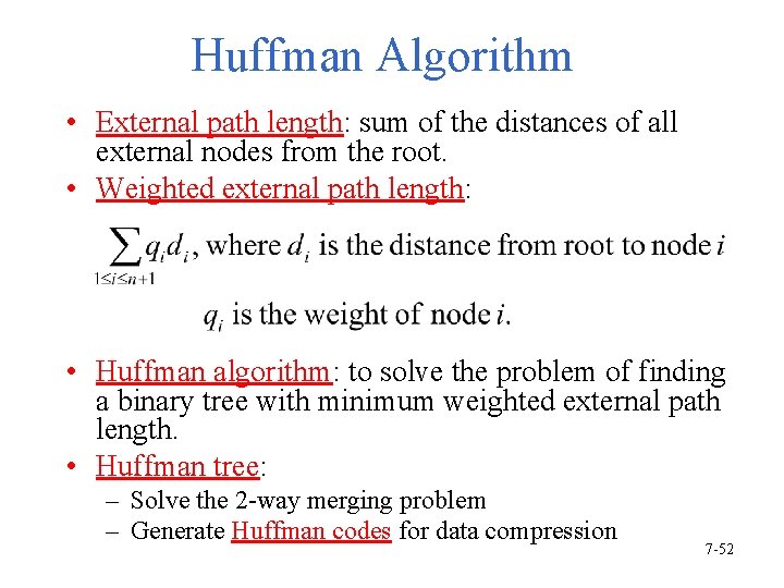
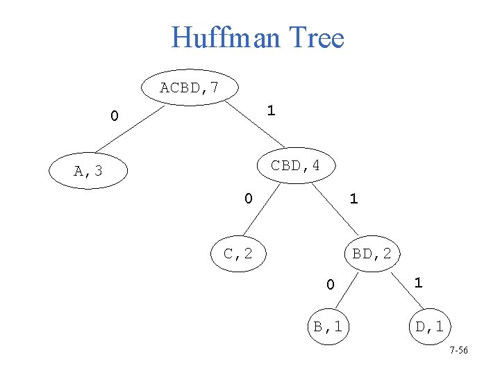
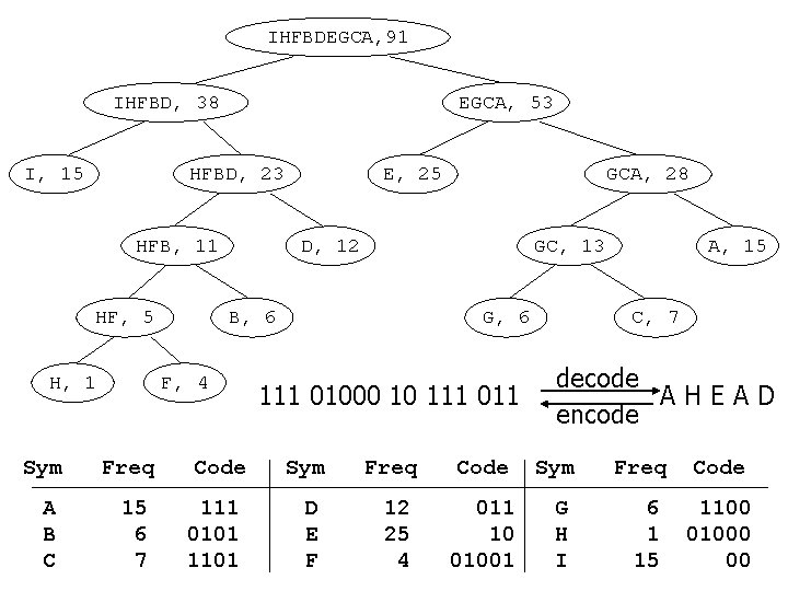
Huffman Algorithm • External path length: sum of the distances of all external nodes from the root. • Weighted external path length: • Huffman algorithm: to solve the problem of finding a binary tree with minimum weighted external path length. • Huffman tree: – Solve the 2 -way merging problem – Generate Huffman codes for data compression 7 -52
![Construction of Huffman Tree 5 3 2 a 2 3 5 7 9 13 Construction of Huffman Tree 5 3 2 (a) [2, 3, 5, 7, 9, 13]](https://slidetodoc.com/presentation_image_h/11db954aaa85205f333354e3f428e601/image-53.jpg)
Construction of Huffman Tree 5 3 2 (a) [2, 3, 5, 7, 9, 13] 10 2 2 3 (d) [10, 13, 16] (c) [7, 9, 10, 13] 3 39 16 13 5 7 9 5 (b) [5, 5, 7, 9, 13] 23 5 16 10 5 9 Min heap is used. Time: O(n log n) 23 10 7 5 2 (e) [16, 23] 13 5 3 7 -53

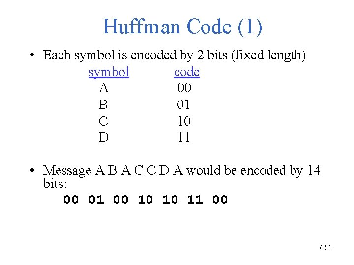
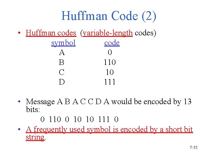
Huffman Code (1) • Each symbol is encoded by 2 bits (fixed length) symbol code A 00 B 01 C 10 D 11 • Message A B A C C D A would be encoded by 14 bits: 00 01 00 10 10 11 00 7 -54

Huffman Code (2) • Huffman codes (variable-length codes) symbol code A 0 B 110 C 10 D 111 • Message A B A C C D A would be encoded by 13 bits: 0 110 0 10 10 111 0 • A frequently used symbol is encoded by a short bit string. 7 -55

Huffman Tree ACBD, 7 1 0 CBD, 4 A, 3 0 1 C, 2 BD, 2 0 B, 1 1 D, 1 7 -56

IHFBDEGCA, 91 IHFBD, 38 I, 15 EGCA, 53 HFBD, 23 HFB, 11 HF, 5 H, 1 Freq A B C 15 6 7 GCA, 28 D, 12 GC, 13 B, 6 F, 4 Sym E, 25 Code 111 0101 1101 G, 6 111 01000 10 111 011 A, 15 C, 7 decode AHEAD encode Sym Freq Code D E F 12 25 4 011 10 01001 G H I 6 1 15 1100 01000 00