Data Structures Chapter 10 Efficient Binary Search Trees

Data Structures Chapter 10: Efficient Binary Search Trees 10 -1

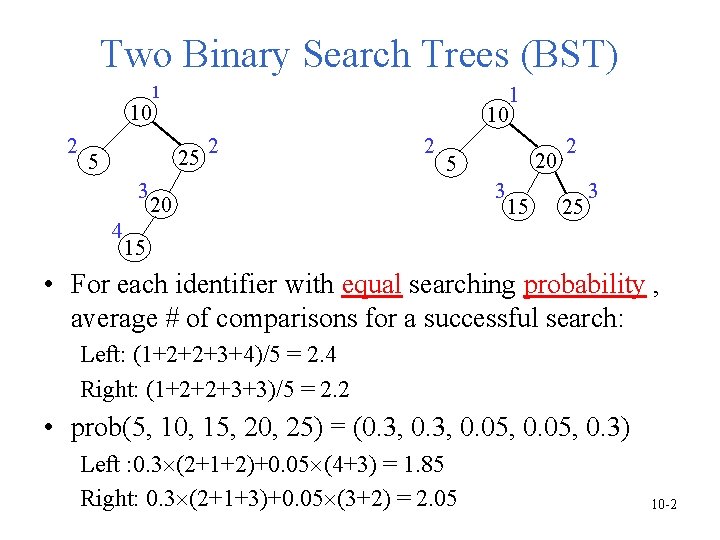
Two Binary Search Trees (BST) 10 2 1 10 25 5 3 4 2 2 1 20 5 20 3 15 2 25 3 15 • For each identifier with equal searching probability , average # of comparisons for a successful search: Left: (1+2+2+3+4)/5 = 2. 4 Right: (1+2+2+3+3)/5 = 2. 2 • prob(5, 10, 15, 20, 25) = (0. 3, 0. 05, 0. 3) Left : 0. 3 (2+1+2)+0. 05 (4+3) = 1. 85 Right: 0. 3 (2+1+3)+0. 05 (3+2) = 2. 05 10 -2

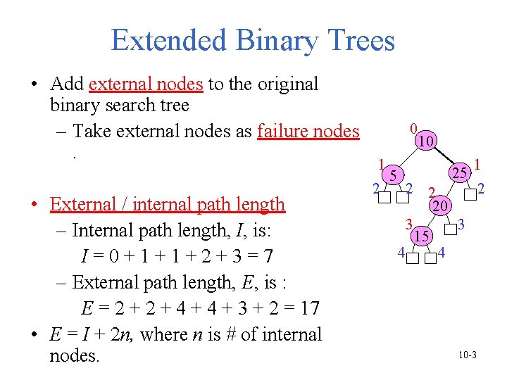
Extended Binary Trees • Add external nodes to the original binary search tree – Take external nodes as failure nodes. • External / internal path length – Internal path length, I, is: I=0+1+1+2+3=7 – External path length, E, is : E = 2 + 4 + 3 + 2 = 17 • E = I + 2 n, where n is # of internal nodes. 0 1 2 5 10 25 1 2 20 3 3 15 4 4 10 -3

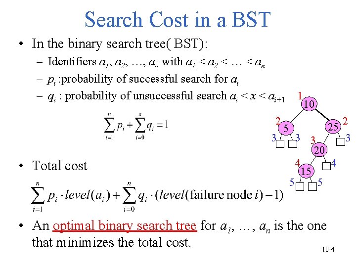
Search Cost in a BST • In the binary search tree( BST): – Identifiers a 1, a 2, …, an with a 1 < a 2 < … < an – pi : probability of successful search for ai – qi : probability of unsuccessful search ai < x < ai+1 2 3 • Total cost 5 1 10 25 2 3 3 3 20 4 4 15 5 5 • An optimal binary search tree for a 1, …, an is the one that minimizes the total cost. 10 -4

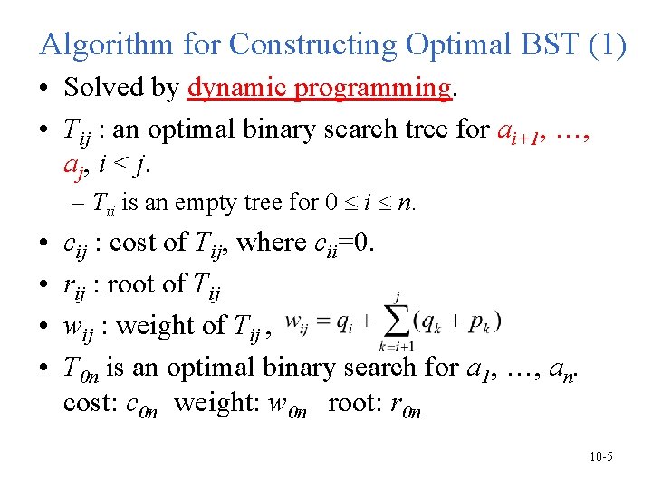
Algorithm for Constructing Optimal BST (1) • Solved by dynamic programming. • Tij : an optimal binary search tree for ai+1, …, aj, i < j. – Tii is an empty tree for 0 i n. • • cij : cost of Tij, where cii=0. rij : root of Tij wij : weight of Tij , T 0 n is an optimal binary search for a 1, …, an. cost: c 0 n weight: w 0 n root: r 0 n 10 -5

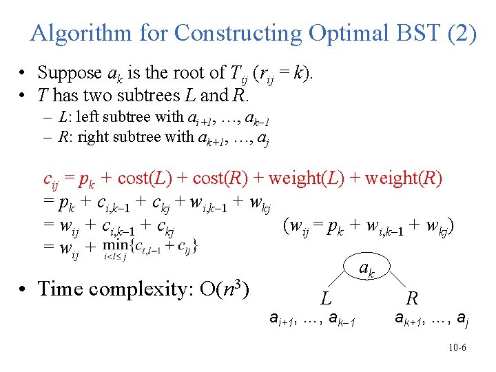
Algorithm for Constructing Optimal BST (2) • Suppose ak is the root of Tij (rij = k). • T has two subtrees L and R. – L: left subtree with ai+1, …, ak 1 – R: right subtree with ak+1, …, aj cij = pk + cost(L) + cost(R) + weight(L) + weight(R) = pk + ci, k 1 + ckj + wi, k 1 + wkj = wij + ci, k 1 + ckj (wij = pk + wi, k 1 + wkj) = wij + ak • Time complexity: O(n 3) L ai+1, …, ak 1 R ak+1, …, aj 10 -6

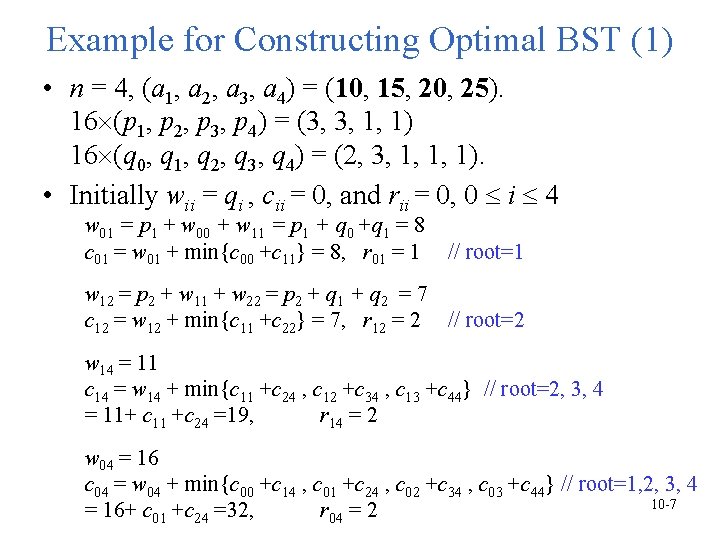
Example for Constructing Optimal BST (1) • n = 4, (a 1, a 2, a 3, a 4) = (10, 15, 20, 25). 16 (p 1, p 2, p 3, p 4) = (3, 3, 1, 1) 16 (q 0, q 1, q 2, q 3, q 4) = (2, 3, 1, 1, 1). • Initially wii = qi , cii = 0, and rii = 0, 0 i 4 w 01 = p 1 + w 00 + w 11 = p 1 + q 0 +q 1 = 8 c 01 = w 01 + min{c 00 +c 11} = 8, r 01 = 1 // root=1 w 12 = p 2 + w 11 + w 22 = p 2 + q 1 + q 2 = 7 c 12 = w 12 + min{c 11 +c 22} = 7, r 12 = 2 // root=2 w 14 = 11 c 14 = w 14 + min{c 11 +c 24 , c 12 +c 34 , c 13 +c 44} // root=2, 3, 4 = 11+ c 11 +c 24 =19, r 14 = 2 w 04 = 16 c 04 = w 04 + min{c 00 +c 14 , c 01 +c 24 , c 02 +c 34 , c 03 +c 44} // root=1, 2, 3, 4 10 -7 = 16+ c 01 +c 24 =32, r 04 = 2

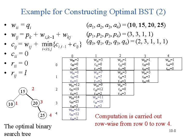
Example for Constructing Optimal BST (2) • • • wii = qi wij = pk + wi, k 1 + wkj cij = wij + cii = 0 0 w =2 c =0 rii = 0 0 r =0 w =8 rij = l c =8 1 00 00 00 01 01 15 10 1 2 2 20 3 3 25 4 The optimal binary search tree 4 r 01=1 w 02=12 c 02=19 r 02=1 w 03=14 c 03=25 r 03=2 w 04=16 c 04=32 r 04=2 (a 1, a 2, a 3, a 4) = (10, 15, 20, 25) (p 1, p 2, p 3, p 4) = (3, 3, 1, 1) (q 0, q 1, q 2, q 3, q 4) = (2, 3, 1, 1, 1) 1 w 11=3 c 11=0 r 11=0 w 12=7 c 12=7 r 12=2 w 13=9 c 13=12 r 13=2 w 14=11 c 14=19 r 14=2 2 w 22=1 c 22=0 r 22=0 w 23=3 c 23=3 r 23=3 w 24=5 c 24=8 r 24=3 3 w 33=1 c 33=0 r 33=0 w 34=3 c 34=3 r 34=4 4 w 44=1 c 44=0 r 44=0 Computation is carried out row-wise from row 0 to row 4. 10 -8

AVL Trees • Height balanced binary search trees. • Proposed by G. Adelson-Velsky and E. M. Landis • Balance factor of each node v – BF(v) =h. L h. R = 1, 0, or 1 – h. L: height of left subtree – h. R: height of right subtree • We can insert an element into the tree, or delete an element from it, in O(log n) time. • At most one single rotation or double rotation is needed when an insertion is performed. 10 -9

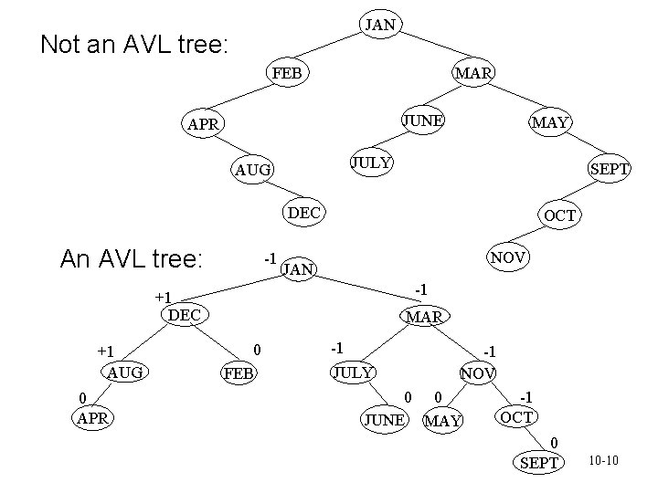
JAN Not an AVL tree: FEB MAR JUNE APR MAY JULY AUG SEPT DEC An AVL tree: -1 OCT NOV JAN -1 +1 DEC +1 AUG 0 APR MAR 0 FEB -1 JULY -1 NOV 0 0 JUNE MAY -1 OCT 0 SEPT 10 -10

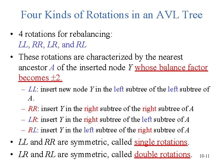
Four Kinds of Rotations in an AVL Tree • 4 rotations for rebalancing: LL, RR, LR, and RL • These rotations are characterized by the nearest ancestor A of the inserted node Y whose balance factor becomes 2. – LL: insert new node Y in the left subtree of A. – RR: insert Y in the right subtree of A – LR: insert Y in the right subtree of the left subtree of A – RL: insert Y in the left subtree of the right subtree of A • LL and RR are symmetric, called single rotations. • LR and RL are symmetric, called double rotations. 10 -11

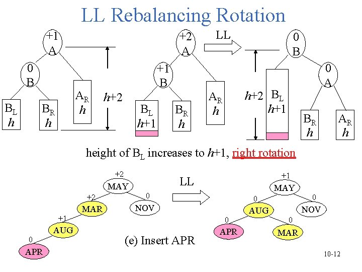
LL Rebalancing Rotation +1 A 0 B BL h +2 A AR h BR h +1 B h+2 BL h+1 BR h LL 0 B 0 A h+2 BL h+1 AR h BR h AR h height of BL increases to h+1, right rotation +2 MAY +2 +1 0 APR AUG MAR +1 LL MAY 0 0 NOV 0 (e) Insert APR 0 NOV AUG 0 MAR 10 -12

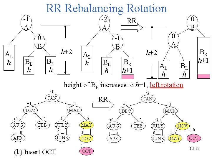
RR Rebalancing Rotation -1 A -2 A 0 B AL h h+2 AL h BR h BL h +1 -1 DEC MAR RR -1 -2 JULY MAY 0 -1 JUNE NOV 0 FEB 0 APR (k) Insert OCT BR h+1 BL h BR h+1 h+2 AL h BL h -1 JAN AUG 0 A -1 B height of BR increases to h+1, left rotation -1 +1 0 B RR 0 OCT JAN +1 +1 0 DEC MAR -1 0 JULY NOV 0 AUG 0 APR FEB 0 0 JUNE MAY 0 OCT 10 -13

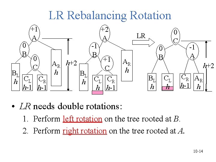
LR Rebalancing Rotation 0 B +1 A 0 C BL h CL CR h-1 -1 B AR h h+2 +2 A +1 C BL h CL CR h h-1 0 C LR AR h 0 B -1 A h+2 BL h C R AR h-1 h • LR needs double rotations: 1. Perform left rotation on the tree rooted at B. 2. Perform right rotation on the tree rooted at A. 10 -14

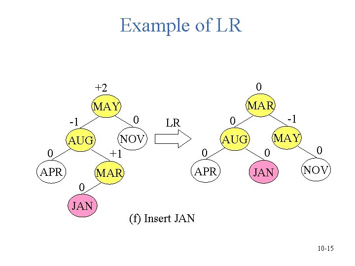
Example of LR 0 +2 MAY -1 0 AUG APR MAR 0 0 LR NOV +1 MAR 0 APR -1 MAY AUG 0 JAN 0 NOV 0 JAN (f) Insert JAN 10 -15

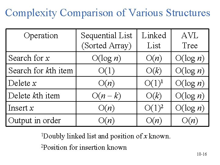
Complexity Comparison of Various Structures Operation Sequential List (Sorted Array) Search for x O(log n) Search for kth item O(1) Delete x O(n) Delete kth item O(n k) Insert x O(n) Output in order O(n) 1 Doubly Linked List O(n) O(k) O(1)1 O(k) O(1)2 O(n) AVL Tree O(log n) O(log n) O(n) linked list and position of x known. 2 Position for insertion known 10 -16

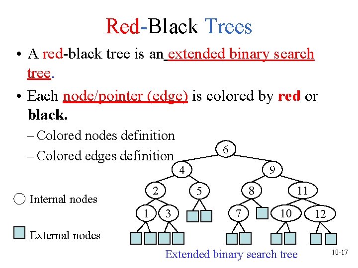
Red-Black Trees • A red-black tree is an extended binary search tree. • Each node/pointer (edge) is colored by red or black. – Colored nodes definition – Colored edges definition 6 4 2 Internal nodes 1 9 8 5 3 7 11 10 12 External nodes Extended binary search tree 10 -17

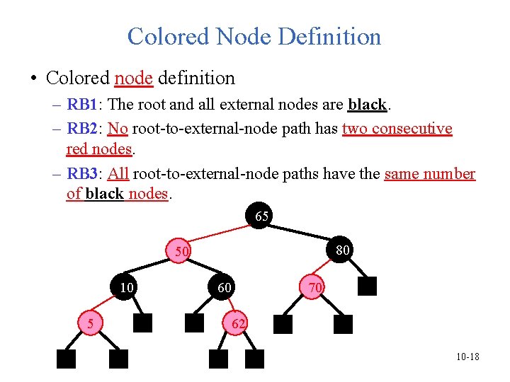
Colored Node Definition • Colored node definition – RB 1: The root and all external nodes are black. – RB 2: No root-to-external-node path has two consecutive red nodes. – RB 3: All root-to-external-node paths have the same number of black nodes. 65 80 50 10 5 60 70 62 10 -18

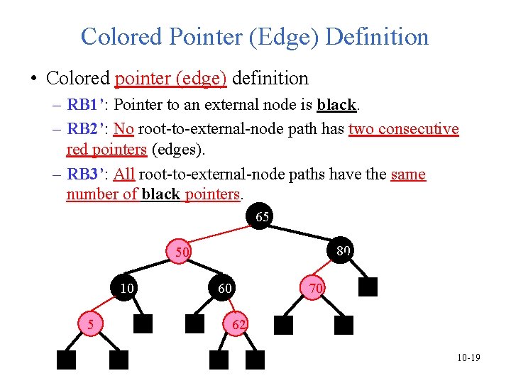
Colored Pointer (Edge) Definition • Colored pointer (edge) definition – RB 1’: Pointer to an external node is black. – RB 2’: No root-to-external-node path has two consecutive red pointers (edges). – RB 3’: All root-to-external-node paths have the same number of black pointers. 65 80 50 10 5 60 70 62 10 -19

Length and Rank in a Red-Black Tree • Let the length of a root-to-external-node path be the number of pointers (edges) on the path. • Let the rank of a node be the number of black pointers (edges) on any path from the node to any external node in its subtree. • Lemma: P, Q: two root-to-external-node paths length(P) 2 * length (Q) • Proof: Let the rank of the root be r. – From RB 2’, each red pointer is followed by a black pointer. – Therefore, each root-to-external-node path has between r and 2 r pointers. 10 -20

Properties of a Red-Black Tree • Lemma: Let h be the height of a red-black tree (excluding the external nodes), let n be the number of internal nodes, and let r be the rank of the root. (a) h 2 r (b) n 2 r 1 (c) h 2 log 2(n+1) • Proof: (a) is correct by previous lemma. From (b), we have r log 2(n+1). This inequality together with (a) yields (c). • Height of a red-black tree 2 log 2(n+1), searching, insertion, and deletion needs O(log n) time. 10 -21

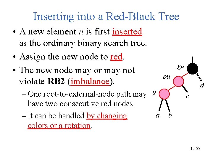
Inserting into a Red-Black Tree • A new element u is first inserted as the ordinary binary search tree. • Assign the new node to red. • The new node may or may not violate RB 2 (imbalance). – One root-to-external-node path may u have two consecutive red nodes. a – It can be handled by changing colors or a rotation. gu pu d c b 10 -22

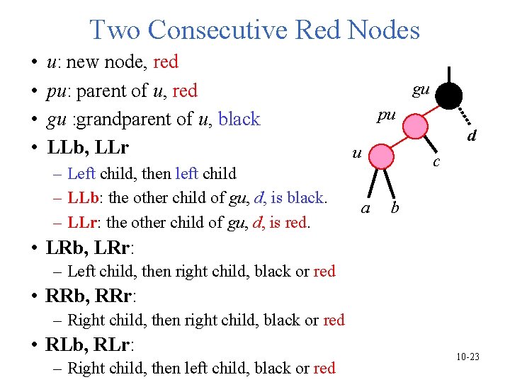
Two Consecutive Red Nodes • • u: new node, red pu: parent of u, red gu : grandparent of u, black LLb, LLr – Left child, then left child – LLb: the other child of gu, d, is black. – LLr: the other child of gu, d, is red. gu pu d u c a b • LRb, LRr: – Left child, then right child, black or red • RRb, RRr: – Right child, then right child, black or red • RLb, RLr: – Right child, then left child, black or red 10 -23

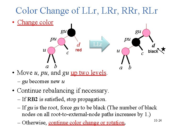
Color Change of LLr, LRr, RLr • Change color gu gu pu u a d c LLr red b • Move u, pu, and gu up two levels. pu d u a c black b – gu becomes new u • Continue rebalancing if necessary. – If RB 2 is satisfied, stop propagation. – If gu is the root, force gu to be black (The number of black nodes on all root-to-external-node paths increases by 1. ) 10 -24 – Otherwise, continue color change or rotation.

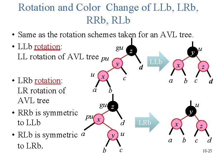
Rotation and Color Change of LLb, LRb, RLb • Same as the rotation schemes taken for an AVL tree. • LLb rotation: gu z y u LL rotation of AVL tree pu y u x c • LRb rotation: a b LR rotation of AVL tree gu z • RRb is symmetric pu x d to LLb • RLb is symmetric a y u to LRb. c b d LLb x a z b c y LRb u x a d z b c d 10 -25

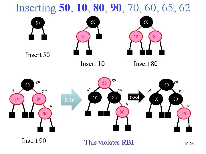
Inserting 50, 10, 80, 90, 70, 65, 62 50 50 50 10 10 80 Insert 10 Insert 80 Insert 50 50 gu d 50 d pu 10 80 u 90 Insert 90 gu RRr 50 pu 10 gu d root 80 u 90 This violates RB 1 pu 10 80 u 90 10 -26

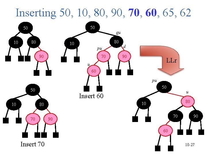
Inserting 50, 10, 80, 90, 70, 65, 62 50 50 10 80 gu 80 10 pu 90 70 d 90 LLr u 60 pu 50 50 10 u Insert 60 70 80 10 80 70 90 90 60 Insert 70 10 -27

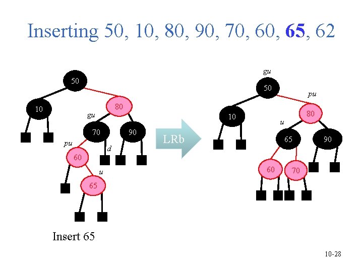
Inserting 50, 10, 80, 90, 70, 65, 62 gu 50 10 50 pu 80 gu 10 70 pu 90 d 80 u LRb 65 90 60 u 60 70 65 Insert 65 10 -28

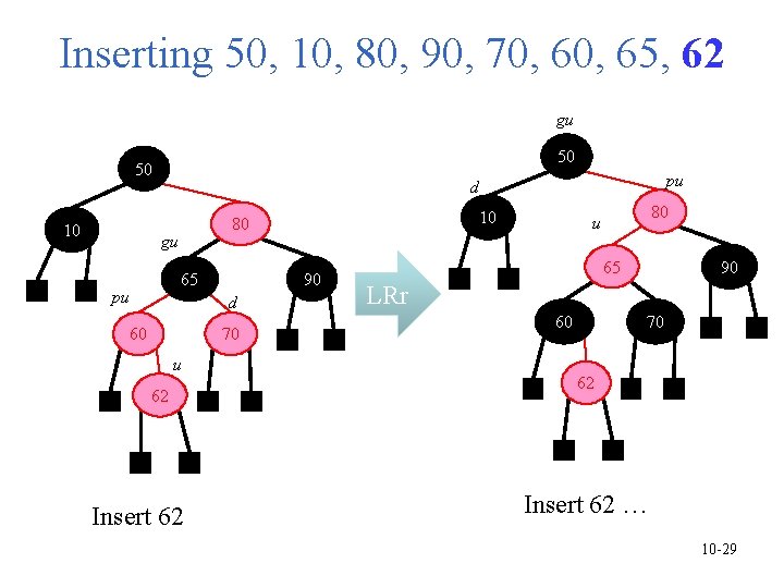
Inserting 50, 10, 80, 90, 70, 65, 62 gu 50 50 10 pu d gu 65 pu 10 80 90 d 60 70 u 62 Insert 62 80 u 65 90 LRr 60 70 62 Insert 62 … 10 -29

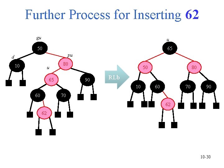
Further Process for Inserting 62 gu u 50 65 pu d 10 u 80 65 50 90 RLb 10 60 80 60 70 90 70 62 62 10 -30

Splay Trees 斜張樹/伸展樹 • A splay tree is a binary search tree. • In an AVL tree, we have to store the balance factor. In a red-black tree, we have store the red/black color. • In a splay tree, there is no balanced information. • The operation for searching, insertion or deletion needs O(log n) amortized time. (worst case O(n). ) • Two variants – Bottom-up splay tree 10 -31

Bottom-Up Splay Trees • Searching, insertion and deletion are performed as in an unbalanced binary search tree, then followed by a splay operation (a sequence of rotations). • The start node x for the splay: – The searched, inserted node – The parent of the deleted node. • After the splay operation completes, the splay node x becomes the tree root. 10 -32

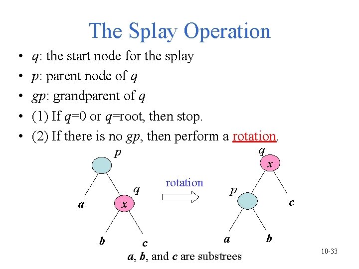
The Splay Operation • • • q: the start node for the splay p: parent node of q gp: grandparent of q (1) If q=0 or q=root, then stop. (2) If there is no gp, then perform a rotation. q p x q rotation p c x a b a c a, b, and c are substrees b 10 -33

Rotations in the Splay Operation • (3) If q has a parent p and a grandparent gp, then a rotation is performed: – – LL: left child, left child RR: right child, right child LR; left child, right child RL: right child, left child • Move up 2 levels at a time. • The splay is repeated at the new location of q, until q becomes the root. • LL and RR are symmetric. LR and RL are 10 -34 symmetric.

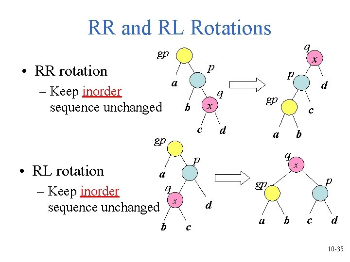
RR and RL Rotations q gp p • RR rotation – Keep inorder sequence unchanged a c gp • RL rotation x b p q c a b q p x p gp q – Keep inorder x sequence unchanged b d gp d a x d c a b c d 10 -35

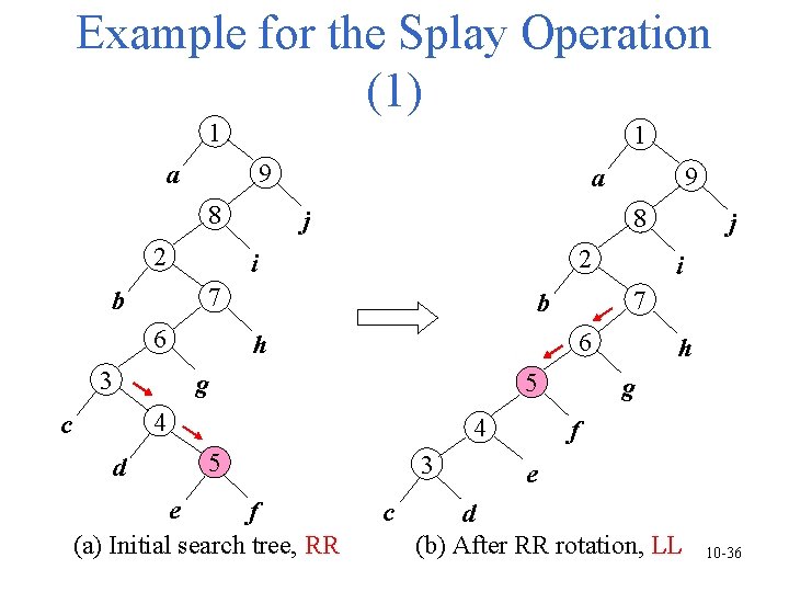
Example for the Splay Operation (1) 1 1 9 a 8 2 8 j 2 i 7 b 6 3 5 4 d 4 5 e f (a) Initial search tree, RR i 6 h 3 c j 7 b g c 9 a h g f e d (b) After RR rotation, LL 10 -36

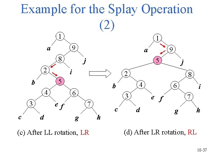
Example for the Splay Operation (2) 1 1 9 a 8 2 5 i 4 3 c j 8 4 b 6 ef d j 2 5 b 9 a 3 7 g (c) After LL rotation, LR c h 6 e f d i 7 g h (d) After LR rotation, RL 10 -37

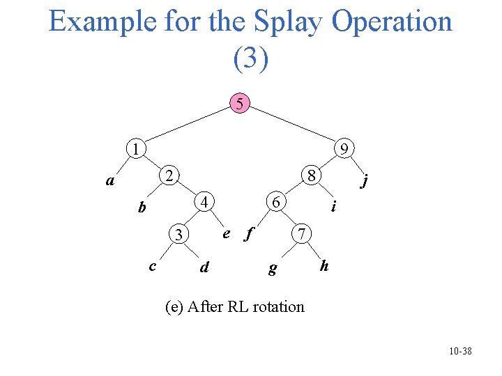
Example for the Splay Operation (3) 5 9 1 8 2 a 6 4 b e f 3 c d j i 7 g h (e) After RL rotation 10 -38

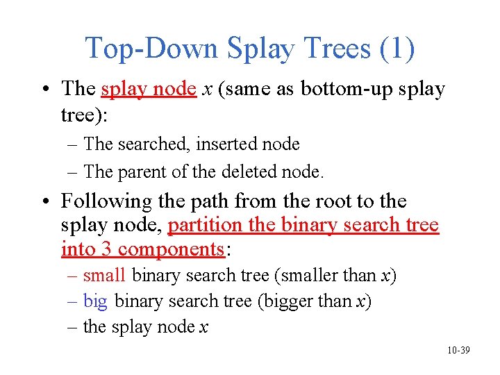
Top-Down Splay Trees (1) • The splay node x (same as bottom-up splay tree): – The searched, inserted node – The parent of the deleted node. • Following the path from the root to the splay node, partition the binary search tree into 3 components: – small binary search tree (smaller than x) – big binary search tree (bigger than x) – the splay node x 10 -39

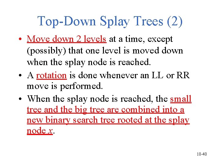
Top-Down Splay Trees (2) • Move down 2 levels at a time, except (possibly) that one level is moved down when the splay node is reached. • A rotation is done whenever an LL or RR move is performed. • When the splay node is reached, the small tree and the big tree are combined into a new binary search tree rooted at the splay node x. 10 -40

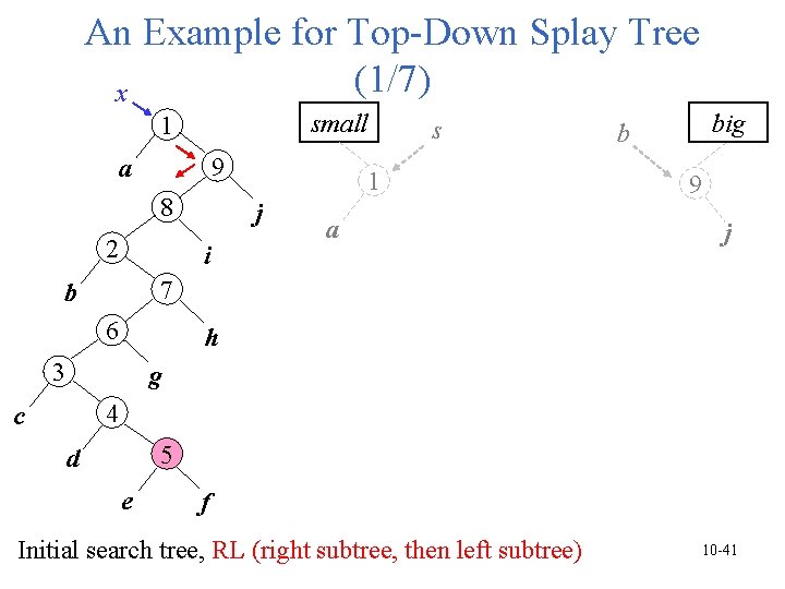
An Example for Top-Down Splay Tree (1/7) x small 1 9 a 8 2 1 j i s a big b 9 j 7 b 6 h 3 g 4 c 5 d e f Initial search tree, RL (right subtree, then left subtree) 10 -41

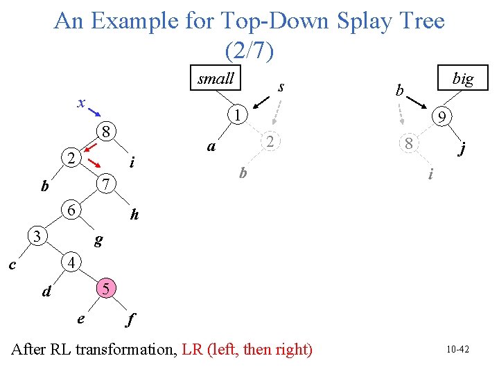
An Example for Top-Down Splay Tree (2/7) small x i 7 b 6 big b 1 8 2 s 9 2 a b 8 j i h 3 g 4 c 5 d e f After RL transformation, LR (left, then right) 10 -42

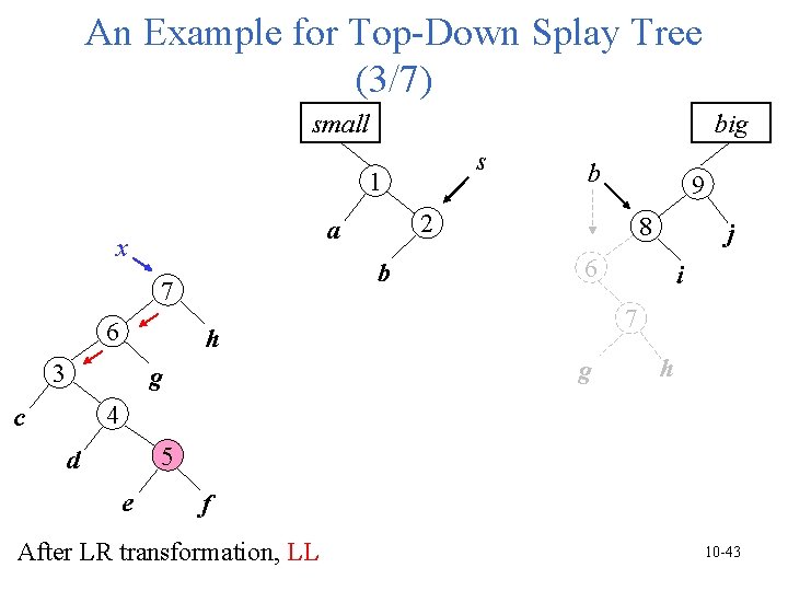
An Example for Top-Down Splay Tree (3/7) small big s 1 b 7 6 8 i 7 g g j 6 h 3 9 2 a x b h 4 c 5 d e f After LR transformation, LL 10 -43

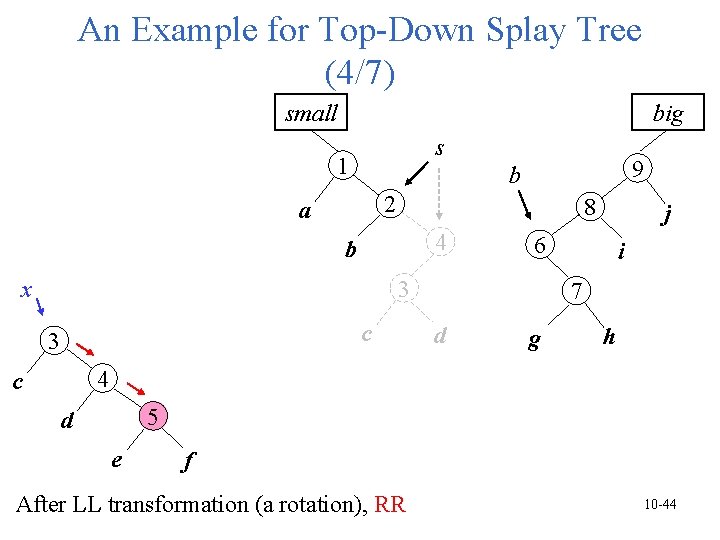
An Example for Top-Down Splay Tree (4/7) small big s 1 9 b 2 a 8 4 b 6 3 x c 3 j i 7 d g h 4 c 5 d e f After LL transformation (a rotation), RR 10 -44

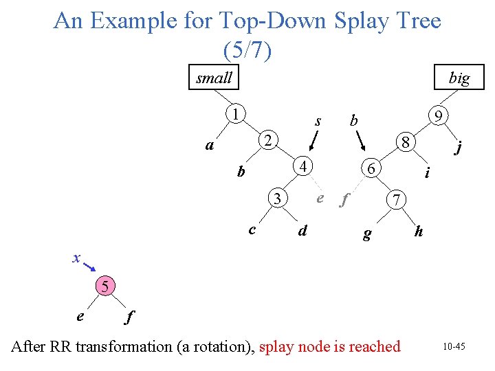
An Example for Top-Down Splay Tree (5/7) small big 1 s 9 b 2 a 8 4 b c 6 e 3 d j f i 7 g h x 5 e f After RR transformation (a rotation), splay node is reached 10 -45

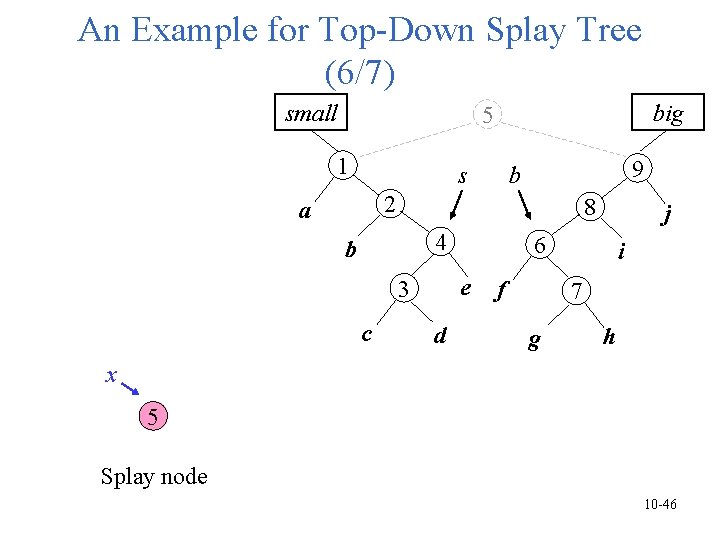
An Example for Top-Down Splay Tree (6/7) small big 5 1 s 9 b 2 a 8 4 b c 6 e 3 d j f i 7 g h x 5 Splay node 10 -46

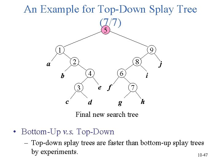
An Example for Top-Down Splay Tree (7/7) 5 9 1 8 2 a 6 4 b e f 3 c j d i 7 g h Final new search tree • Bottom-Up v. s. Top-Down – Top-down splay trees are faster than bottom-up splay trees by experiments. 10 -47