Data Structures and Algorithm Analysis and Sorting Lecturer

Data Structures and Algorithm Analysis and Sorting Lecturer: Jing Liu Email: neouma@mail. xidian. edu. cn Homepage: http: //see. xidian. edu. cn/faculty/liujing

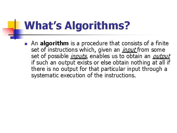
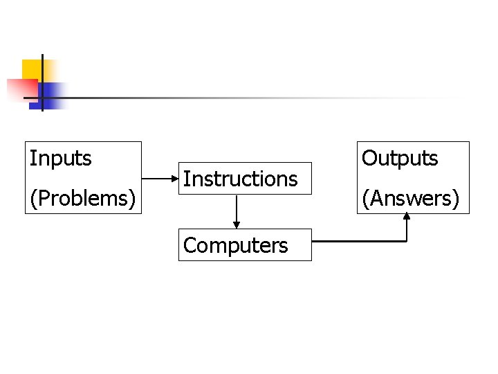
What’s Algorithms? n An algorithm is a procedure that consists of a finite set of instructions which, given an input from some set of possible inputs, enables us to obtain an output if such an output exists or else obtain nothing at all if there is no output for that particular input through a systematic execution of the instructions.

Inputs (Problems) Instructions Computers Outputs (Answers)

Programming Languages Data Structure Algorithms Software Systems

Binary Search n Let A[1…n] be a sequence of n elements. Consider the problem of determining whether a given element x is in A.

Binary Search Example: A[1… 14]=1 4 5 7 8 9 10 12 15 22 23 27 32 35 x=22 Does x exist in A? How many comparisons do you need to give the answer?

Binary Search n n n n n Inputs: (1) An array A[1…n] of n elements sorted in nondecreasing order; (2) x; Output: j if x=A[j], and 0 otherwise; 1. 2. 3. 4. 5. 6. 7. 8. low 1; high n; j 0; while (low high) and (j=0) mid (low+high)/2 ; if x=A[mid] then j mid; else if x<A[mid] then high mid– 1; else low mid+1; end while; return j;

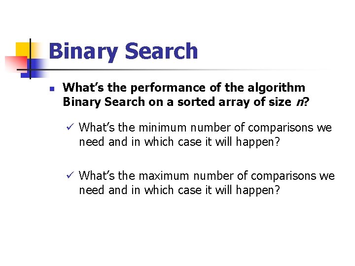
Binary Search n What’s the performance of the algorithm Binary Search on a sorted array of size n? ü What’s the minimum number of comparisons we need and in which case it will happen? ü What’s the maximum number of comparisons we need and in which case it will happen?

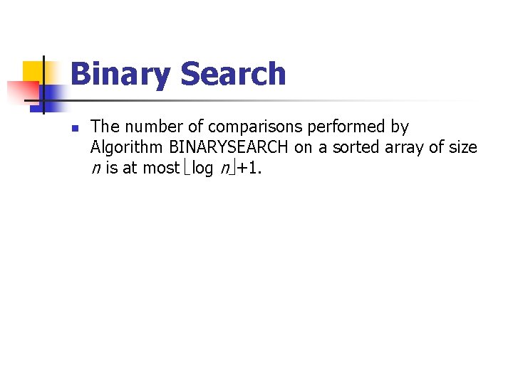
Binary Search n The number of comparisons performed by Algorithm BINARYSEARCH on a sorted array of size n is at most log n +1.

Binary Search n Can you implement the Binary Search in a certain kind of computer language?

Merging Two Sorted Lists n Suppose we have an array A[1…m] and three indices p, q, and r, with 1 p q<r m, such that both the subarrays A[p…q] and A[q+1…r] are individually sorted in nondecreasing order. We want to rearrange the elements in A so that the elements in the subarray A[p…r] are sorted in nondecreasing order.

Merging Two Sorted Lists Example: A[1… 7]=5 8 11 4 8 10 12 p=1, q=3, r=7 A[1… 3] and A[4… 7] are already sorted nondecreasingly, please sort A nondecreasingly? How many comparisons do you need to give the answer?

Merging Two Sorted Lists n n Inputs: (1) A[1…m]; (2) p, q, and r, and 1 p q<r m, such that both A[p…q] and A[q+1…r] are sorted individually in nondecreasing order; Output: A[p…r] contains the result of merging the two subarrays A[p…q] and A[q+1…r];

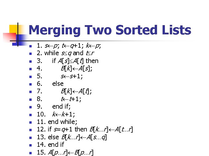
Merging Two Sorted Lists n n n n 1. s p; t q+1; k p; 2. while s q and t r 3. if A[s] A[t] then 4. B[k] A[s]; 5. s s+1; 6. else 7. B[k] A[t]; 8. t t+1; 9. end if; 10. k k+1; 11. end while; 12. if s=q+1 then B[k…r] A[t…r] 13. else B[k…r] A[s…q] 14. end if 15. A[p…r] B[p…r]

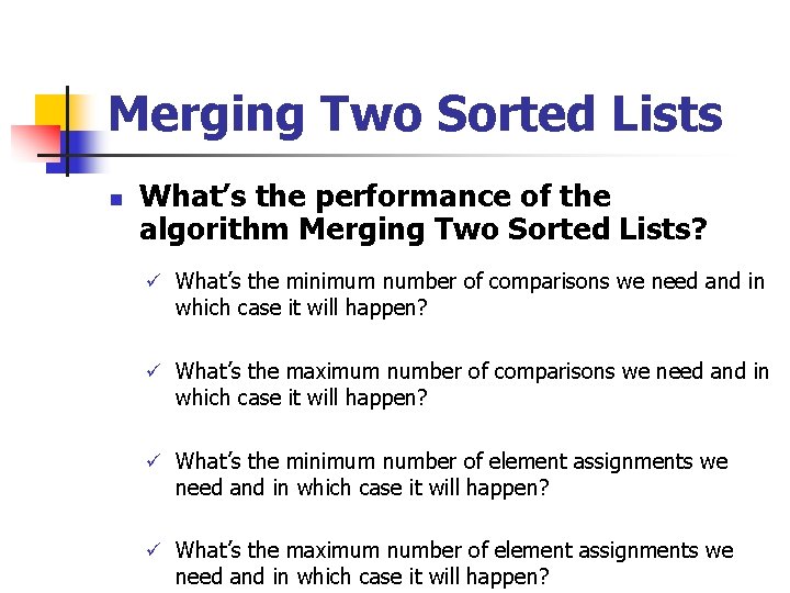
Merging Two Sorted Lists n What’s the performance of the algorithm Merging Two Sorted Lists? ü What’s the minimum number of comparisons we need and in which case it will happen? ü What’s the maximum number of comparisons we need and in which case it will happen? ü What’s the minimum number of element assignments we need and in which case it will happen? ü What’s the maximum number of element assignments we need and in which case it will happen?

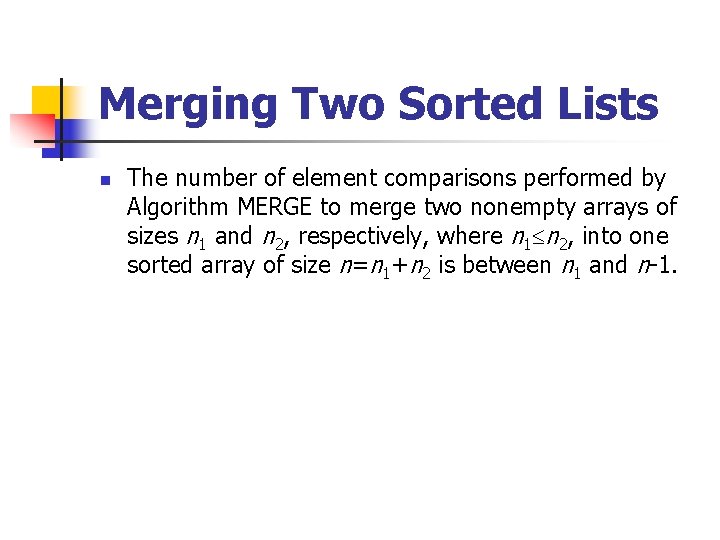
Merging Two Sorted Lists n The number of element comparisons performed by Algorithm MERGE to merge two nonempty arrays of sizes n 1 and n 2, respectively, where n 1 n 2, into one sorted array of size n=n 1+n 2 is between n 1 and n-1.

Merging Two Sorted Lists n The number of element assignments performed by Algorithm MERGE to merge two arrays into one sorted array of size n is exactly 2 n.

Problems and Algorithms n Each algorithm is designed to solve one problem, but for one problem, we can design many different algorithms. ü What’s the difference of these algorithms? ü Why we design different algorithms for the same problem? Example Problem: Sort ü Selection Sort ü Insertion Sort ü Bottom-Up Merge Sorting

Selection Sort n n n Let A[1…n] be an array of n elements. A simple and straightforward algorithm to sort the entries in A works as follows. First, we find the minimum element and store it in A[1]. Next, we find the minimum of the remaining n-1 elements and store it in A[2]. We continue this way until the second largest element is stored in A[n-1].

Selection Sort n n n n n Input: A[1…n]; Output: A[1…n] sorted in nondecreasing order; 1. for i 1 to n-1 2. k i ; 3. for j i+1 to n 4. if A[j]<A[k] then k j; 5. end for; 6. if k i then interchange A[i] and A[k]; 7. end for;

Selection Sort n What’s the performance of the algorithm Selection Sort? ü What’s the minimum number of comparisons we need and in which case it will happen? ü What’s the maximum number of comparisons we need and in which case it will happen? ü What’s the minimum number of element assignments? ü What’s the maximum number of element assignments?

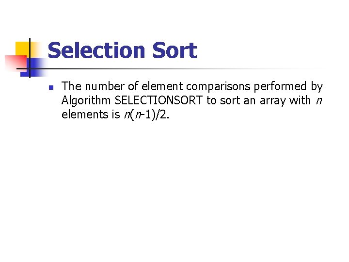
Selection Sort n The number of element comparisons performed by Algorithm SELECTIONSORT to sort an array with n elements is n(n-1)/2.

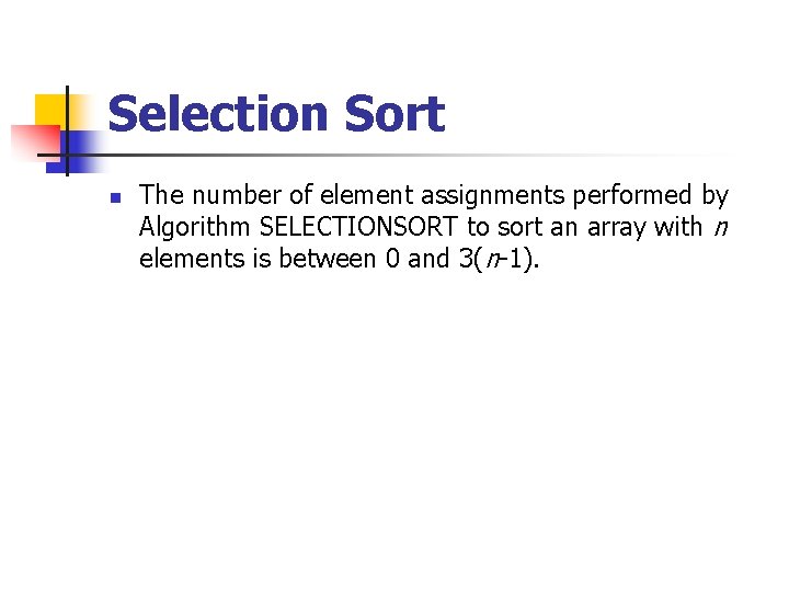
Selection Sort n The number of element assignments performed by Algorithm SELECTIONSORT to sort an array with n elements is between 0 and 3(n-1).

Insertion Sort n n We begin with the subarray of size 1, A[1], which is already sorted. Next, A[2] is inserted before or after A[1] depending on whether it is smaller than A[1] or not. Continuing this way, in the i th iteration, A[i] is inserted in its proper position in the sorted subarray A[1 … i-1]. This is done by scanning the elements from index i-1 down to 1, each time comparing A[i] with the element at the current position.

Insertion Sort n n In each iteration of the scan, an element is shifted one position up to a higher index. This process of scanning, performing the comparison and shifting continues until an element less than or equal to A[i] is found, or when all the sorted sequence so far is exhausted. At this point, A[i] is inserted in its proper position, and the process of inserting element A[i] in its proper place is complete.

Insertion Sort Example: A[1 … 4]=9 4 5 2

Insertion Sort n n n Input: An array A[1…n] of n elements; Output: A[1…n] sorted in nondecreasing order; 1. for i 2 to n 2. x A[i]; 3. j i-1; 4. while (j>0) and (A[j]>x) 5. A[j+1] A[j]; 6. j j-1; 7. end while; 8. A[j+1] x; 9. end for;

Insertion Sort n What’s the performance of the algorithm Insertion Sort? ü What’s the minimum number of comparisons we need and in which case it will happen? ü What’s the maximum number of comparisons we need and in which case it will happen? ü What’s the minimum number of element assignments? ü What’s the maximum number of element assignments?

Insertion Sort n The number of element comparisons performed by Algorithm INSERTIONSORT is between n-1 and n(n-1)/2.

Insertion Sort n The number of element assignments performed by Algorithm INSERTIONSORT is equal to the number of element comparisons plus n-1.

Bottom-Up Merge Sorting Example: A[1 … 8]=9 4 5 2 1 7 4 6

Bottom-Up Merge Sorting Example: A[1 … 11]=6 10 9 5 3 11 4 8 1 2 7

Bottom-Up Merge Sorting n n n Let A be an array of n elements that is to be sorted. We first merge n/2 consecutive pairs of elements to yield n/2 sorted sequences of size 2. If there is one remaining element, then it is passed to the next iteration. Next, we merge n/4 pairs of consecutive 2 -element sequences to yield n/4 sorted sequences of size 4. If there are one or two remaining elements, then they are passed to the next iteration. If there are three elements left, then two (sorted) elements are merged with one element to form a 3 element sorted sequence.

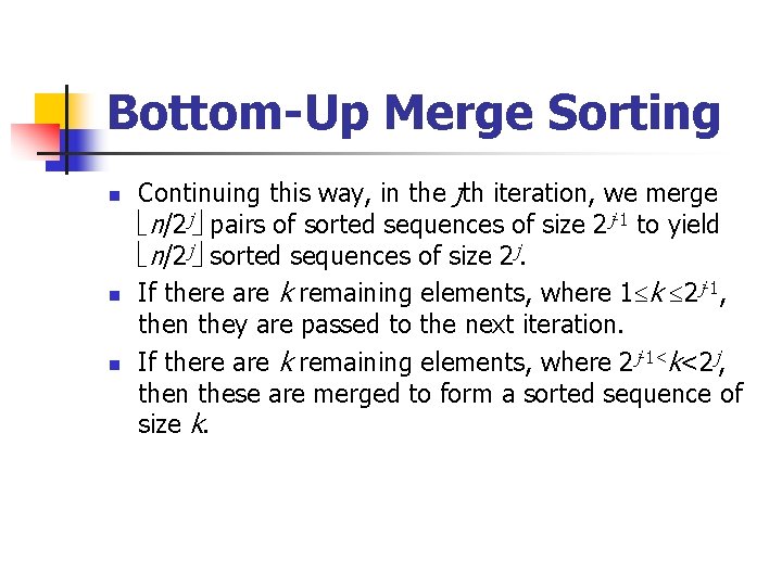
Bottom-Up Merge Sorting n n n Continuing this way, in the jth iteration, we merge n/2 j pairs of sorted sequences of size 2 j-1 to yield n/2 j sorted sequences of size 2 j. If there are k remaining elements, where 1 k 2 j-1, then they are passed to the next iteration. If there are k remaining elements, where 2 j-1<k<2 j, then these are merged to form a sorted sequence of size k.

Bottom-Up Merge Sorting n n n Input: An array A[1…n] of n elements; Output: A[1…n] sorted in nondecreasing order; 1. t 1; 2. while t<n 3. s t; t 2 s; i 0; 4. while i+t n 5. MERGE(A, i+1, i+s, i+t); 6. i i+t; 7. end while; 8. if i+s<n then MERGE(A, i+1, i+s, n); 9. end while;

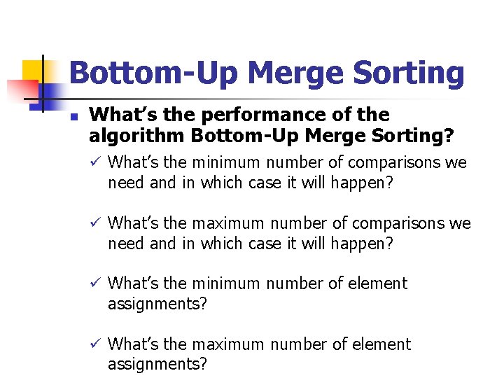
Bottom-Up Merge Sorting n What’s the performance of the algorithm Bottom-Up Merge Sorting? ü What’s the minimum number of comparisons we need and in which case it will happen? ü What’s the maximum number of comparisons we need and in which case it will happen? ü What’s the minimum number of element assignments? ü What’s the maximum number of element assignments?

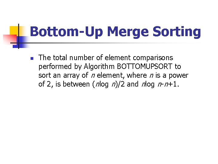
Bottom-Up Merge Sorting n The total number of element comparisons performed by Algorithm BOTTOMUPSORT to sort an array of n element, where n is a power of 2, is between (nlog n)/2 and nlog n-n+1.

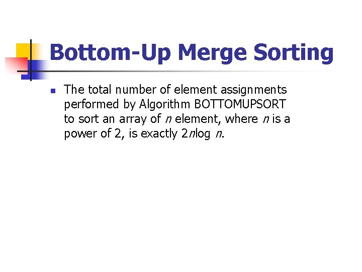
Bottom-Up Merge Sorting n The total number of element assignments performed by Algorithm BOTTOMUPSORT to sort an array of n element, where n is a power of 2, is exactly 2 nlog n.

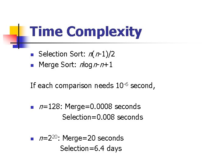
Time Complexity n n Selection Sort: n(n-1)/2 Merge Sort: nlogn-n+1 If each comparison needs 10 -6 second, n n=128: Merge=0. 0008 seconds Selection=0. 008 seconds n n=220: Merge=20 seconds Selection=6. 4 days

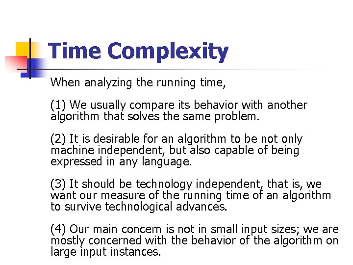
Time Complexity When analyzing the running time, (1) We usually compare its behavior with another algorithm that solves the same problem. (2) It is desirable for an algorithm to be not only machine independent, but also capable of being expressed in any language. (3) It should be technology independent, that is, we want our measure of the running time of an algorithm to survive technological advances. (4) Our main concern is not in small input sizes; we are mostly concerned with the behavior of the algorithm on large input instances.

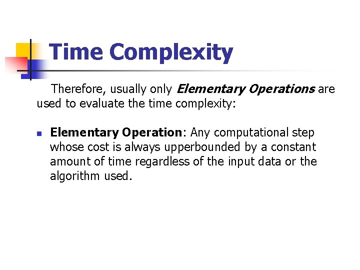
Time Complexity Therefore, usually only Elementary Operations are used to evaluate the time complexity: n Elementary Operation: Any computational step whose cost is always upperbounded by a constant amount of time regardless of the input data or the algorithm used.

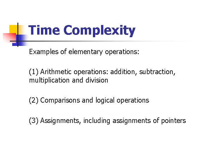
Time Complexity Examples of elementary operations: (1) Arithmetic operations: addition, subtraction, multiplication and division (2) Comparisons and logical operations (3) Assignments, including assignments of pointers

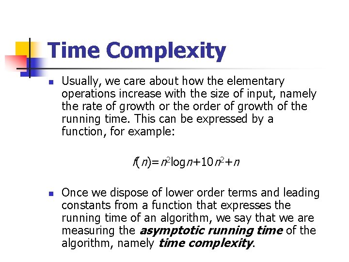
Time Complexity n Usually, we care about how the elementary operations increase with the size of input, namely the rate of growth or the order of growth of the running time. This can be expressed by a function, for example: f(n)=n 2 logn+10 n 2+n n Once we dispose of lower order terms and leading constants from a function that expresses the running time of an algorithm, we say that we are measuring the asymptotic running time of the algorithm, namely time complexity.

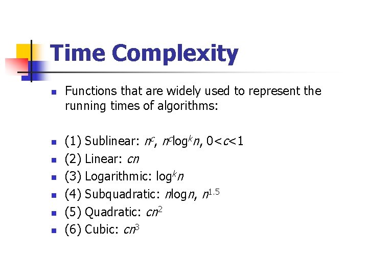
Time Complexity n n n n Functions that are widely used to represent the running times of algorithms: (1) (2) (3) (4) (5) (6) Sublinear: nc, nclogkn, 0<c<1 Linear: cn Logarithmic: logkn Subquadratic: nlogn, n 1. 5 Quadratic: cn 2 Cubic: cn 3

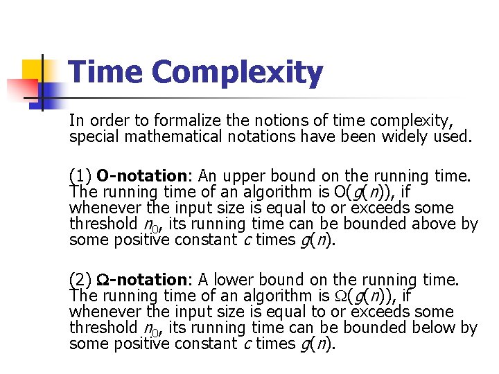
Time Complexity In order to formalize the notions of time complexity, special mathematical notations have been widely used. (1) O-notation: An upper bound on the running time. The running time of an algorithm is O(g(n)), if whenever the input size is equal to or exceeds some threshold n 0, its running time can be bounded above by some positive constant c times g(n). (2) -notation: A lower bound on the running time. The running time of an algorithm is (g(n)), if whenever the input size is equal to or exceeds some threshold n 0, its running time can be bounded below by some positive constant c times g(n).

Time Complexity (3) -notation: An exact bound. The running time of an algorithm is of order (g(n)) if whenever the input size is equal to or exceeds some threshold n 0, its running time can be bounded below by c 1 g(n) and above by c 2 g(n), where 0<c 1 c 2.

Time Complexity (1) f(n) is (g(n)) if and only if g(n) is O(f(n)) (2) f(n)= (g(n)) if and only if f(n)=O(g(n)) and f(n)= (g(n))

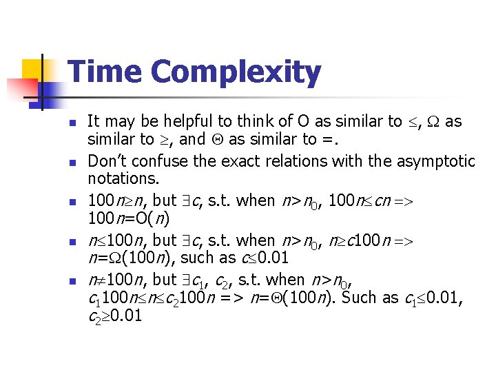
Time Complexity n n n It may be helpful to think of O as similar to , and as similar to =. Don’t confuse the exact relations with the asymptotic notations. 100 n n, but c, s. t. when n>n 0, 100 n cn 100 n=O(n) n 100 n, but c, s. t. when n>n 0, n c 100 n n= (100 n), such as c 0. 01 n 100 n, but c 1, c 2, s. t. when n>n 0, c 1100 n n c 2100 n => n= (100 n). Such as c 1 0. 01, c 2 0. 01

Time Complexity n How to use the notations O, , to represent the time complexity of the three previous sorting algorithms?

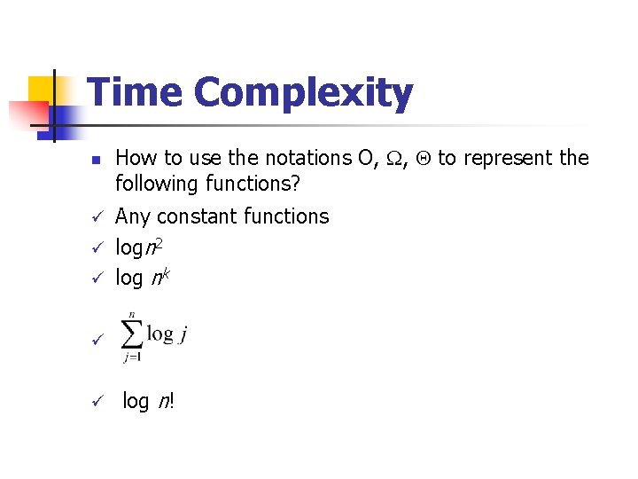
Time Complexity n How to use the notations O, , to represent the following functions? Any constant functions ü logn 2 ü log nk ü ü ü log n!

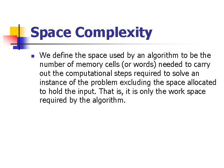
Space Complexity n We define the space used by an algorithm to be the number of memory cells (or words) needed to carry out the computational steps required to solve an instance of the problem excluding the space allocated to hold the input. That is, it is only the work space required by the algorithm.

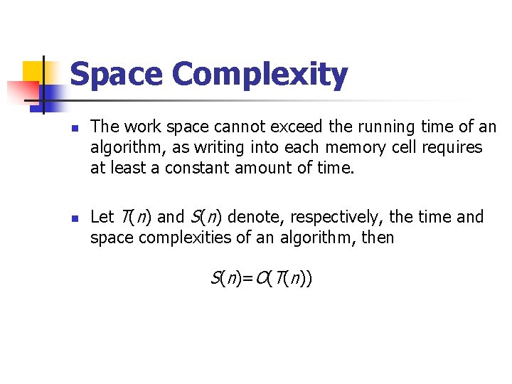
Space Complexity n n The work space cannot exceed the running time of an algorithm, as writing into each memory cell requires at least a constant amount of time. Let T(n) and S(n) denote, respectively, the time and space complexities of an algorithm, then S(n)=O(T(n))

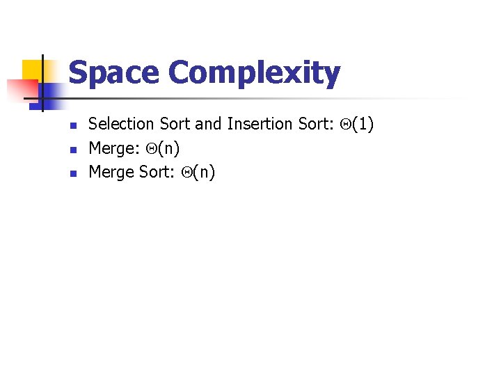
Space Complexity n n n Selection Sort and Insertion Sort: (1) Merge: (n) Merge Sort: (n)

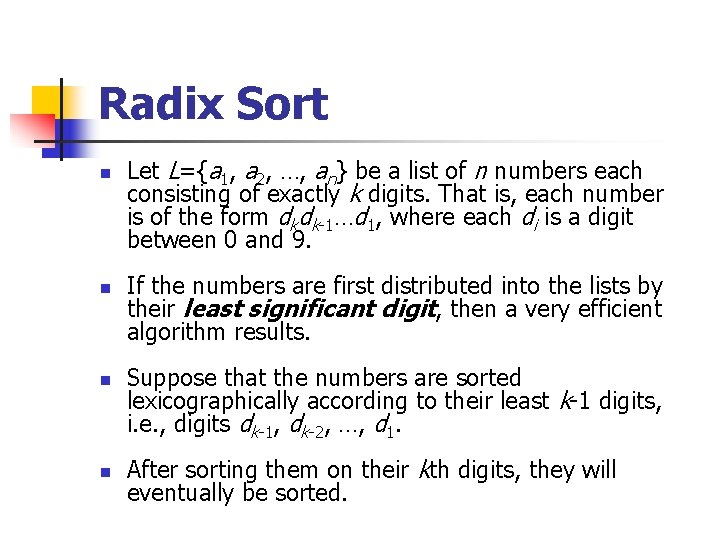
Radix Sort n n Let L={a 1, a 2, …, an} be a list of n numbers each consisting of exactly k digits. That is, each number is of the form dkdk-1…d 1, where each di is a digit between 0 and 9. If the numbers are first distributed into the lists by their least significant digit, then a very efficient algorithm results. Suppose that the numbers are sorted lexicographically according to their least k-1 digits, i. e. , digits dk-1, dk-2, …, d 1. After sorting them on their kth digits, they will eventually be sorted.

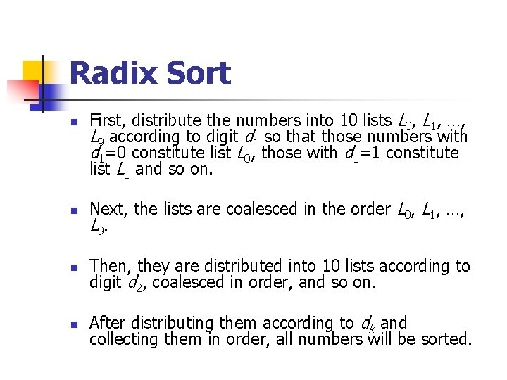
Radix Sort n n First, distribute the numbers into 10 lists L 0, L 1, …, L 9 according to digit d 1 so that those numbers with d 1=0 constitute list L 0, those with d 1=1 constitute list L 1 and so on. Next, the lists are coalesced in the order L 0, L 1, …, L 9. Then, they are distributed into 10 lists according to digit d 2, coalesced in order, and so on. After distributing them according to dk and collecting them in order, all numbers will be sorted.

Radix Sort Example: Sort A nondecreasingly. A[1… 5]=7467 3275 6792 9134 1239

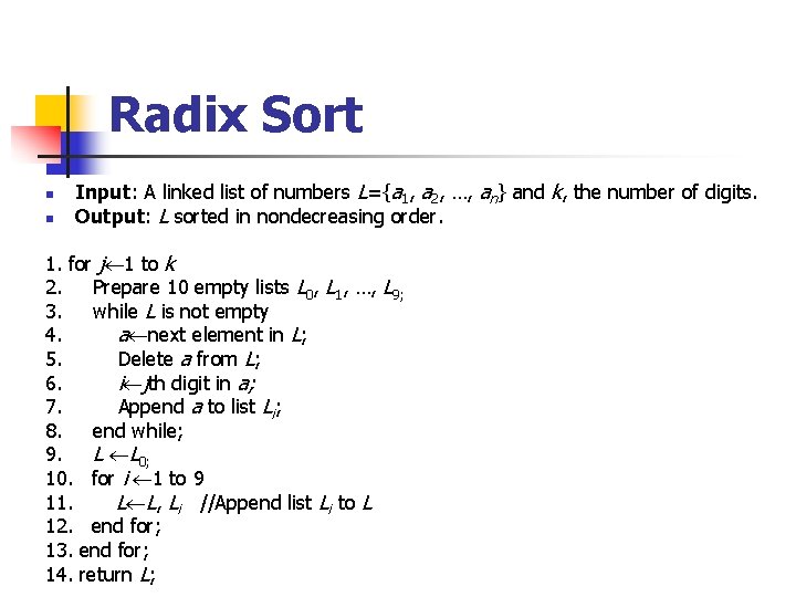
Radix Sort n n Input: A linked list of numbers L={a 1, a 2, …, an} and k, the number of digits. Output: L sorted in nondecreasing order. 1. for j 1 to k 2. Prepare 10 empty lists L 0, L 1, …, L 9; 3. while L is not empty 4. a next element in L; 5. Delete a from L; 6. i jth digit in a; 7. Append a to list Li; 8. end while; 9. L L 0; 10. for i 1 to 9 11. L L, Li //Append list Li to L 12. end for; 13. end for; 14. return L;

Radix Sort n What’s the performance of the algorithm Radix Sort? ü Time Complexity? ü Space Complexity?

Radix Sort n Time Complexity: (n) n Space Complexity: (n)

Radix Sort n Write codes to implement the Radix Sort.

Quicksort n n n Let A[low…high] be an array of n numbers, and x=A[low]. We consider the problem of rearranging the elements in A so that all elements less than or equal to x precede x which in turn precedes all elements greater than x. After permuting the element in the array, x will be A[w] for some w, low w high. The action of rearrangement is also called splitting or partitioning around x, which is called the pivot or splitting element.

Quicksort n n We say that an element A[j] is in its proper position or correct position if it is neither smaller than the elements in A[low…j-1] nor larger than the elements in A[j+1…high]. After partitioning an array A using x A as a pivot, x will be in its correct position.

Quicksort n n n n Input: An array of elements A[low…high]; Output: (1) A with its elements rearranged, if necessary; (2) w, the new position of the splitting element A[low]; 1. i low; 2. x A[low]; 3. for j low+1 to high 4. if A[j] x then 5. i i+1; 6. if i j then interchange A[i] and A[j]; 7. end if; 8. end for; 9. interchange A[low] and A[i]; 10. w i; 11. return A and w;

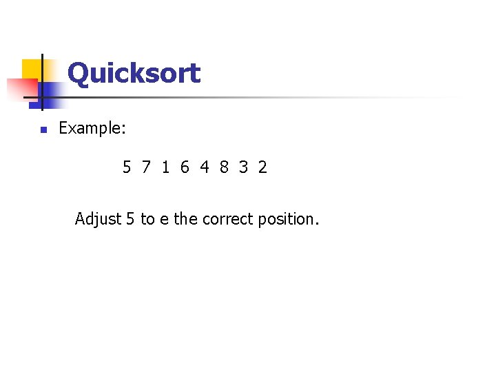
Quicksort n Example: 5 7 1 6 4 8 3 2 Adjust 5 to e the correct position.

Quicksort n n The number of element comparisons performed by Algorithm SPLIT is exactly n-1. Thus, its time complexity is (n). The only extra space used is that needed to hold its local variables. Therefore, the space complexity is (1).

Quicksort n Input: An array A[1…n] of n elements; Output: The elements in A sorted in nondecreasing order; n 1. quicksort(A, 1, n); n n n n quicksort(A, low, high) 1. if low<high then 2. SPLIT(A[low…high], w) \w is the new position of A[low]; 3. quicksort(A, low, w-1); 4. quicksort(A, w+1, high); 5. end if;

Quicksort n The average number of comparisons performed by Algorithm QUICKSORT to sort an array of n elements is (nlogn).

Quicksort n Write codes to implement the Quicksort.

Homework n n Exercises: 7. 13 Implement Quicksort in C