Data Structures Algorithms Lecture Shortest Paths Networks and

Data Structures & Algorithms Lecture: Shortest Paths

Networks and other graphs road network computer network execution order for processes process 4 process 1 process 3 process 2 process 5 process 6

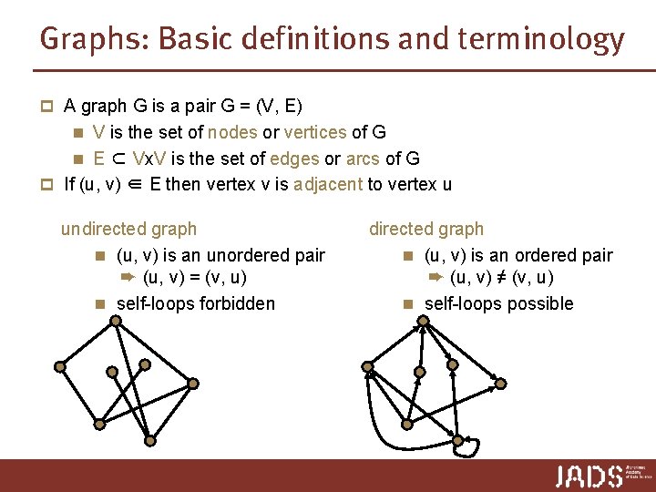
Graphs: Basic definitions and terminology p A graph G is a pair G = (V, E) n V is the set of nodes or vertices of G n E ⊂ Vx. V is the set of edges or arcs of G p If (u, v) ∈ E then vertex v is adjacent to vertex u undirected graph n (u, v) is an unordered pair ➨ (u, v) = (v, u) n self-loops forbidden directed graph n (u, v) is an ordered pair ➨ (u, v) ≠ (v, u) n self-loops possible

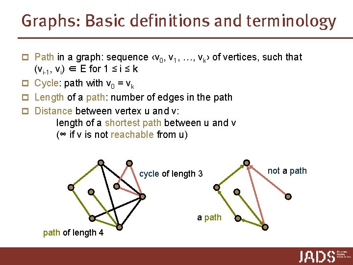
Graphs: Basic definitions and terminology p Path in a graph: sequence ‹v 0, v 1, …, vk› of vertices, such that (vi-1, vi) ∈ E for 1 ≤ i ≤ k p Cycle: path with v 0 = vk p Length of a path: number of edges in the path p Distance between vertex u and v: length of a shortest path between u and v (∞ if v is not reachable from u) cycle of length 3 a path of length 4 not a path

Single-source shortest path Dijkstra’s algorithm

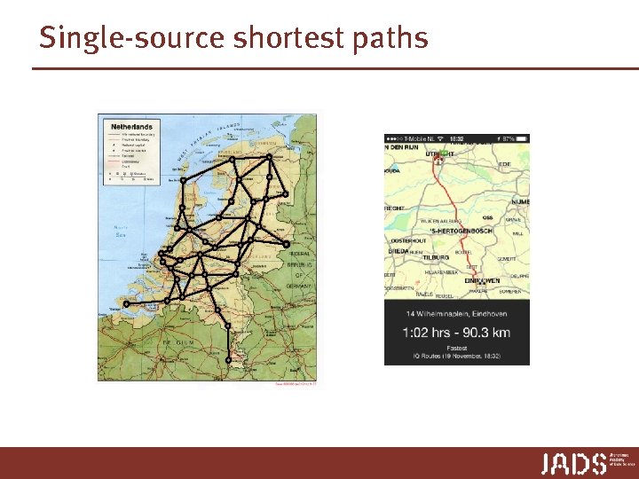
Single-source shortest paths

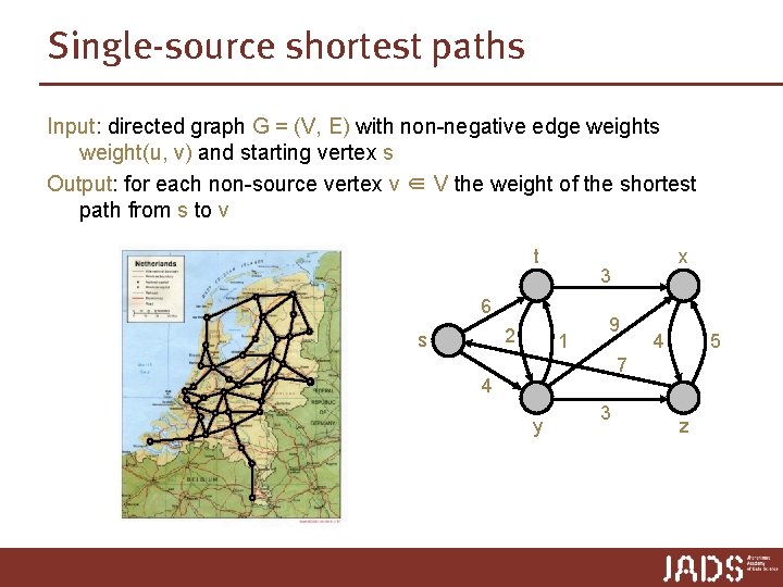
Single-source shortest paths Input: directed graph G = (V, E) with non-negative edge weights weight(u, v) and starting vertex s Output: for each non-source vertex v ∈ V the weight of the shortest path from s to v t 3 6 2 s x 1 9 4 5 7 4 y 3 z

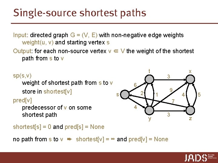
Single-source shortest paths Input: directed graph G = (V, E) with non-negative edge weights weight(u, v) and starting vertex s Output: for each non-source vertex v ∈ V the weight of the shortest path from s to v sp(s, v) weight of shortest path from s to v store in shortest[v] s pred[v] predecessor of v on some shortest path t 3 6 2 x 9 1 4 5 7 4 y 3 shortest[s] = 0 and pred[s] = None no path from s to v ➨ shortest[v] = ∞ and pred[v] = None z

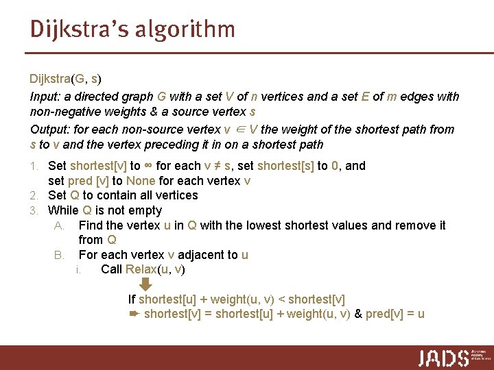
Dijkstra’s algorithm Dijkstra(G, s) Input: a directed graph G with a set V of n vertices and a set E of m edges with non-negative weights & a source vertex s Output: for each non-source vertex v ∈ V the weight of the shortest path from s to v and the vertex preceding it in on a shortest path 1. Set shortest[v] to ∞ for each v ≠ s, set shortest[s] to 0, and set pred [v] to None for each vertex v 2. Set Q to contain all vertices 3. While Q is not empty A. Find the vertex u in Q with the lowest shortest values and remove it from Q B. For each vertex v adjacent to u i. Call Relax(u, v) If shortest[u] + weight(u, v) < shortest[v] ➨ shortest[v] = shortest[u] + weight(u, v) & pred[v] = u

Dijkstra’s algorithm t Dijkstra(G, s) 1. Set shortest[v] to ∞ for each v ≠ s, set shortest[s] to 0, and set pred [v] to None for each vertex v 2. Set Q to contain all vertices 3. While Q is not empty A. Find the vertex u in Q with the lowest shortest values and remove it from Q B. For each vertex v adjacent to u i. Call Relax(u, v) 1. If shortest[u] + weight(u, v) < shortest[v] ➨ shortest[v] = shortest[u] + weight(u, v) & pred[v] = u 2 s 0 4 3 ∞ 6 x 1 ∞ 9 4 5 7 ∞ y 3 ∞ z

Dijkstra’s algorithm t Dijkstra(G, s) 1. Set shortest[v] to ∞ for each v ≠ s, set shortest[s] to 0, and set pred [v] to None for each vertex v 2. Set Q to contain all vertices 3. While Q is not empty A. Find the vertex u in Q with the lowest shortest values and remove it from Q B. For each vertex v adjacent to u i. Call Relax(u, v) 1. If shortest[u] + weight(u, v) < shortest[v] ➨ shortest[v] = shortest[u] + weight(u, v) & pred[v] = u 2 s 0 4 3 6 6 x 1 ∞ 9 4 5 7 ∞ y 3 ∞ z

Dijkstra’s algorithm t Dijkstra(G, s) 1. Set shortest[v] to ∞ for each v ≠ s, set shortest[s] to 0, and set pred [v] to None for each vertex v 2. Set Q to contain all vertices 3. While Q is not empty A. Find the vertex u in Q with the lowest shortest values and remove it from Q B. For each vertex v adjacent to u i. Call Relax(u, v) 1. If shortest[u] + weight(u, v) < shortest[v] ➨ shortest[v] = shortest[u] + weight(u, v) & pred[v] = u 2 s 0 4 3 6 6 x 1 ∞ 9 4 5 7 ∞ y 3 ∞ z

Dijkstra’s algorithm t Dijkstra(G, s) 1. Set shortest[v] to ∞ for each v ≠ s, set shortest[s] to 0, and set pred [v] to None for each vertex v 2. Set Q to contain all vertices 3. While Q is not empty A. Find the vertex u in Q with the lowest shortest values and remove it from Q B. For each vertex v adjacent to u i. Call Relax(u, v) 1. If shortest[u] + weight(u, v) < shortest[v] ➨ shortest[v] = shortest[u] + weight(u, v) & pred[v] = u 2 s 0 4 3 6 6 x 1 ∞ 9 4 5 7 4 y 3 ∞ z

Dijkstra’s algorithm t Dijkstra(G, s) 1. Set shortest[v] to ∞ for each v ≠ s, set shortest[s] to 0, and set pred [v] to None for each vertex v 2. Set Q to contain all vertices 3. While Q is not empty A. Find the vertex u in Q with the lowest shortest values and remove it from Q B. For each vertex v adjacent to u i. Call Relax(u, v) 1. If shortest[u] + weight(u, v) < shortest[v] ➨ shortest[v] = shortest[u] + weight(u, v) & pred[v] = u 2 s 0 4 3 6 6 x 1 ∞ 9 4 5 7 4 y 3 ∞ z

Dijkstra’s algorithm t Dijkstra(G, s) 1. Set shortest[v] to ∞ for each v ≠ s, set shortest[s] to 0, and set pred [v] to None for each vertex v 2. Set Q to contain all vertices 3. While Q is not empty A. Find the vertex u in Q with the lowest shortest values and remove it from Q B. For each vertex v adjacent to u i. Call Relax(u, v) 1. If shortest[u] + weight(u, v) < shortest[v] ➨ shortest[v] = shortest[u] + weight(u, v) & pred[v] = u 2 s 0 4 3 6 6 x 1 ∞ 9 4 5 7 4 y 3 ∞ z

Dijkstra’s algorithm t Dijkstra(G, s) 1. Set shortest[v] to ∞ for each v ≠ s, set shortest[s] to 0, and set pred [v] to None for each vertex v 2. Set Q to contain all vertices 3. While Q is not empty A. Find the vertex u in Q with the lowest shortest values and remove it from Q B. For each vertex v adjacent to u i. Call Relax(u, v) 1. If shortest[u] + weight(u, v) < shortest[v] ➨ shortest[v] = shortest[u] + weight(u, v) & pred[v] = u 2 s 0 4 3 6 6 x 1 ∞ 9 4 5 7 4 y 3 7 z

Dijkstra’s algorithm t Dijkstra(G, s) 1. Set shortest[v] to ∞ for each v ≠ s, set shortest[s] to 0, and set pred [v] to None for each vertex v 2. Set Q to contain all vertices 3. While Q is not empty A. Find the vertex u in Q with the lowest shortest values and remove it from Q B. For each vertex v adjacent to u i. Call Relax(u, v) 1. If shortest[u] + weight(u, v) < shortest[v] ➨ shortest[v] = shortest[u] + weight(u, v) & pred[v] = u 2 s 0 4 3 6 6 x 1 ∞ 9 4 5 7 4 y 3 7 z

Dijkstra’s algorithm t Dijkstra(G, s) 1. Set shortest[v] to ∞ for each v ≠ s, set shortest[s] to 0, and set pred [v] to None for each vertex v 2. Set Q to contain all vertices 3. While Q is not empty A. Find the vertex u in Q with the lowest shortest values and remove it from Q B. For each vertex v adjacent to u i. Call Relax(u, v) 1. If shortest[u] + weight(u, v) < shortest[v] ➨ shortest[v] = shortest[u] + weight(u, v) & pred[v] = u 2 s 0 4 3 6 6 x 1 13 9 4 5 7 4 y 3 7 z

Dijkstra’s algorithm t Dijkstra(G, s) 1. Set shortest[v] to ∞ for each v ≠ s, set shortest[s] to 0, and set pred [v] to None for each vertex v 2. Set Q to contain all vertices 3. While Q is not empty A. Find the vertex u in Q with the lowest shortest values and remove it from Q B. For each vertex v adjacent to u i. Call Relax(u, v) 1. If shortest[u] + weight(u, v) < shortest[v] ➨ shortest[v] = shortest[u] + weight(u, v) & pred[v] = u 2 s 0 4 3 6 6 x 1 13 9 4 5 7 4 y 3 7 z

Dijkstra’s algorithm t Dijkstra(G, s) 1. Set shortest[v] to ∞ for each v ≠ s, set shortest[s] to 0, and set pred [v] to None for each vertex v 2. Set Q to contain all vertices 3. While Q is not empty A. Find the vertex u in Q with the lowest shortest values and remove it from Q B. For each vertex v adjacent to u i. Call Relax(u, v) 1. If shortest[u] + weight(u, v) < shortest[v] ➨ shortest[v] = shortest[u] + weight(u, v) & pred[v] = u 2 s 0 4 3 5 6 x 1 13 9 4 5 7 4 y 3 7 z

Dijkstra’s algorithm t Dijkstra(G, s) 1. Set shortest[v] to ∞ for each v ≠ s, set shortest[s] to 0, and set pred [v] to None for each vertex v 2. Set Q to contain all vertices 3. While Q is not empty A. Find the vertex u in Q with the lowest shortest values and remove it from Q B. For each vertex v adjacent to u i. Call Relax(u, v) 1. If shortest[u] + weight(u, v) < shortest[v] ➨ shortest[v] = shortest[u] + weight(u, v) & pred[v] = u 2 s 0 4 3 5 6 x 1 13 9 4 5 7 4 y 3 7 z

Dijkstra’s algorithm t Dijkstra(G, s) 1. Set shortest[v] to ∞ for each v ≠ s, set shortest[s] to 0, and set pred [v] to None for each vertex v 2. Set Q to contain all vertices 3. While Q is not empty A. Find the vertex u in Q with the lowest shortest values and remove it from Q B. For each vertex v adjacent to u i. Call Relax(u, v) 1. If shortest[u] + weight(u, v) < shortest[v] ➨ shortest[v] = shortest[u] + weight(u, v) & pred[v] = u 2 s 0 4 3 5 6 x 1 13 9 4 5 7 4 y 3 7 z

Dijkstra’s algorithm t Dijkstra(G, s) 1. Set shortest[v] to ∞ for each v ≠ s, set shortest[s] to 0, and set pred [v] to None for each vertex v 2. Set Q to contain all vertices 3. While Q is not empty A. Find the vertex u in Q with the lowest shortest values and remove it from Q B. For each vertex v adjacent to u i. Call Relax(u, v) 1. If shortest[u] + weight(u, v) < shortest[v] ➨ shortest[v] = shortest[u] + weight(u, v) & pred[v] = u 2 s 0 4 3 5 6 x 1 13 9 4 5 7 4 y 3 7 z

Dijkstra’s algorithm t Dijkstra(G, s) 1. Set shortest[v] to ∞ for each v ≠ s, set shortest[s] to 0, and set pred [v] to None for each vertex v 2. Set Q to contain all vertices 3. While Q is not empty A. Find the vertex u in Q with the lowest shortest values and remove it from Q B. For each vertex v adjacent to u i. Call Relax(u, v) 1. If shortest[u] + weight(u, v) < shortest[v] ➨ shortest[v] = shortest[u] + weight(u, v) & pred[v] = u 2 s 0 4 3 5 6 x 1 8 9 4 5 7 4 y 3 7 z

Dijkstra’s algorithm t Dijkstra(G, s) 1. Set shortest[v] to ∞ for each v ≠ s, set shortest[s] to 0, and set pred [v] to None for each vertex v 2. Set Q to contain all vertices 3. While Q is not empty A. Find the vertex u in Q with the lowest shortest values and remove it from Q B. For each vertex v adjacent to u i. Call Relax(u, v) 1. If shortest[u] + weight(u, v) < shortest[v] ➨ shortest[v] = shortest[u] + weight(u, v) & pred[v] = u 2 s 0 4 3 5 6 x 1 8 9 4 5 7 4 y 3 7 z

Dijkstra’s algorithm t Dijkstra(G, s) 1. Set shortest[v] to ∞ for each v ≠ s, set shortest[s] to 0, and set pred [v] to None for each vertex v 2. Set Q to contain all vertices 3. While Q is not empty A. Find the vertex u in Q with the lowest shortest values and remove it from Q B. For each vertex v adjacent to u i. Call Relax(u, v) 1. If shortest[u] + weight(u, v) < shortest[v] ➨ shortest[v] = shortest[u] + weight(u, v) & pred[v] = u 2 s 0 4 3 5 6 x 1 8 9 4 5 7 4 y 3 7 z

Dijkstra’s algorithm t Dijkstra(G, s) 1. Set shortest[v] to ∞ for each v ≠ s, set shortest[s] to 0, and set pred [v] to None for each vertex v 2. Set Q to contain all vertices 3. While Q is not empty A. Find the vertex u in Q with the lowest shortest values and remove it from Q B. For each vertex v adjacent to u i. Call Relax(u, v) 1. If shortest[u] + weight(u, v) < shortest[v] ➨ shortest[v] = shortest[u] + weight(u, v) & pred[v] = u Correctness? 2 s 0 4 3 5 6 x 1 8 9 4 5 7 4 y 3 7 z

Dijkstra’s algorithm t Dijkstra(G, s) 1. Set shortest[v] to ∞ for each v ≠ s, set shortest[s] to 0, and set pred [v] to None for each vertex v 2. Set Q to contain all vertices 3. While Q is not empty A. Find the vertex u in Q with the lowest shortest values and remove it from Q B. For each vertex v adjacent to u i. Call Relax(u, v) 1. If shortest[u] + weight(u, v) < shortest[v] ➨ shortest[v] = shortest[u] + weight(u, v) & pred[v] = u Correctness? 2 s 0 4 3 5 6 x 1 8 9 4 5 7 4 y 3 7 z Invariant At the start of each iteration of the loop in step 3, shortest[v] = sp(s, v) for each vertex v not in the set Q. That is, for each vertex v not in Q the value of shortest[v] is the weight of a shortest path from s to v.

Dijkstra’s algorithm Dijkstra(G, s) 1. 2. 3. Set shortest[v] to ∞ for each v ≠ s, set shortest[s] to 0, and set pred [v] to None for each vertex v Set Q to contain all vertices While Q is not empty A. Find the vertex u in Q with the lowest shortest values and remove it from Q B. For each vertex v adjacent to u i. Call Relax(u, v) 1. If shortest[u] + weight(u, v) < shortest[v] ➨ shortest[v] = shortest[u] + weight(u, v) & pred[v] = u Running time? n vertices, m edges, m ≤ n 2 1. 2. 3. Θ(n) ? ? loop iterates n times and processes each vertex and edge once ➨ (n+m) …but … how long for n Step 2 n finding u with lowest shortest value n bookkeeping after relax?

Dijkstra’s algorithm Dijkstra(G, s) 1. 2. 3. Set shortest[v] to ∞ for each v ≠ s, set shortest[s] to 0, and set pred [v] to None for each vertex v Set Q to contain all vertices While Q is not empty A. Find the vertex u in Q with the lowest shortest values and remove it from Q B. For each vertex v adjacent to u i. Call Relax(u, v) 1. If shortest[u] + weight(u, v) < shortest[v] ➨ shortest[v] = shortest[u] + weight(u, v) & pred[v] = u Insert(Q, v) Inserts vertex v into set Q Extract-Min(Q) removes and returns vertex with minimum shortest value Decrease-Key(Q, v) performs bookkeeping in Q, records that shortest[v] decreased ➨ abstract data type priority queue

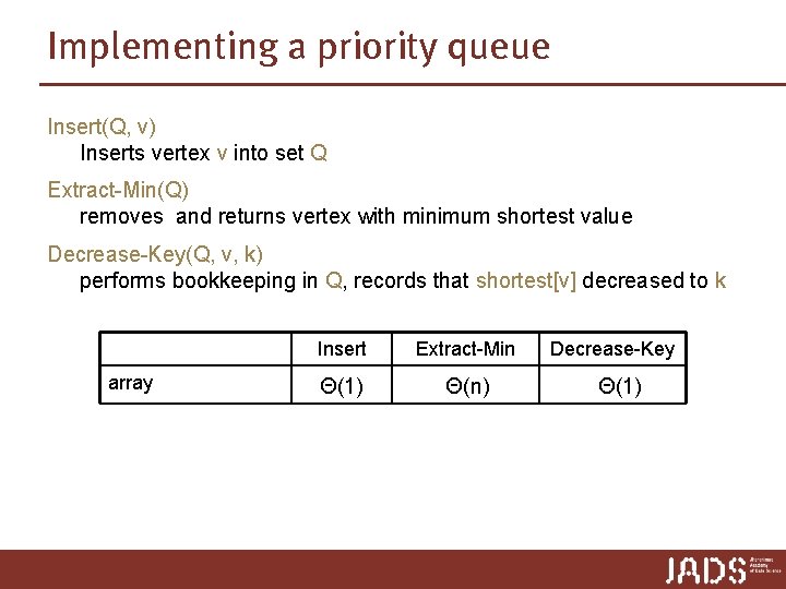
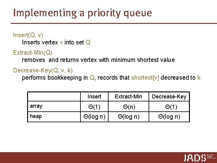
Implementing a priority queue Insert(Q, v) Inserts vertex v into set Q Extract-Min(Q) removes and returns vertex with minimum shortest value Decrease-Key(Q, v, k) performs bookkeeping in Q, records that shortest[v] decreased to k array Insert Extract-Min Θ(1) Θ(n) Decrease-Key Θ(1)

Dijkstra’s algorithm Dijkstra(G, s) 1. Set shortest[v] to ∞ for each v ≠ s, set shortest[s] to 0, and set pred [v] to None for each vertex v 2. Make Q an empty priority queue 3. For each vertex v: A. Call Insert(Q, v) 4. While Q is not empty, do the following A. Call Extract-Min(Q) and set u to hold the returned vertex B. For each vertex v adjacent to u i. Call Relax(u, v) ii. If the call to Relax(u, v) decreased the values of shortest[v], then call Decrease-Key(Q, v) Q implemented by an array ➨ n ∙ Extract-Min(Q) = O(n 2) ➨ Dijkstra O(n 2)

Implementing a priority queue Insert(Q, v) Inserts vertex v into set Q Extract-Min(Q) removes and returns vertex with minimum shortest value Decrease-Key(Q, v, k) performs bookkeeping in Q, records that shortest[v] decreased to k array Insert Extract-Min Θ(1) Θ(n) Decrease-Key Θ(1)

Implementing a priority queue Insert(Q, v) Inserts vertex v into set Q Extract-Min(Q) removes and returns vertex with minimum shortest value Decrease-Key(Q, v, k) performs bookkeeping in Q, records that shortest[v] decreased to k Insert Extract-Min array Θ(1) Θ(n) heap Θ(log n) Decrease-Key Θ(1) Θ(log n)

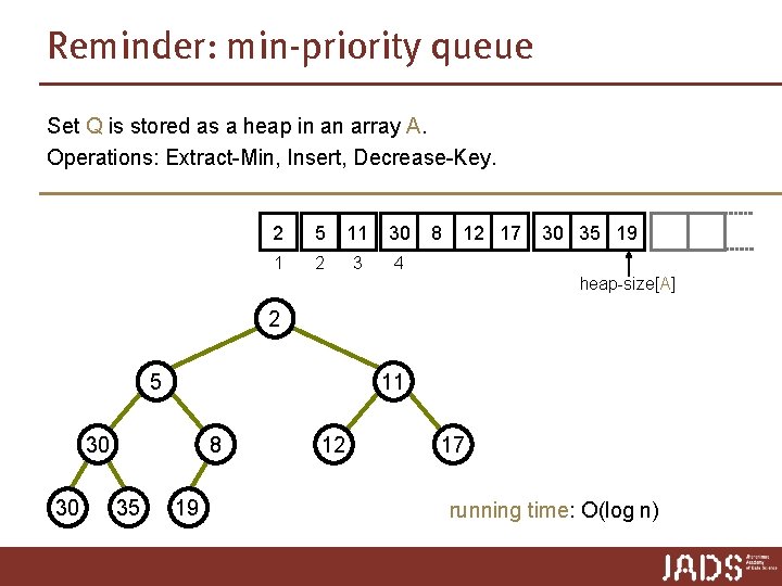
Reminder: min-priority queue Set Q is stored as a heap in an array A. Operations: Extract-Min, Insert, Decrease-Key. 2 5 11 30 1 2 3 4 8 12 17 30 35 19 heap-size[A] 2 5 11 30 30 8 35 19 12 17 running time: O(log n)

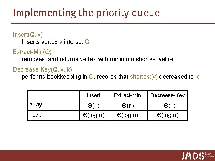
Implementing the priority queue Insert(Q, v) Inserts vertex v into set Q Extract-Min(Q) removes and returns vertex with minimum shortest value Decrease-Key(Q, v, k) performs bookkeeping in Q, records that shortest[v] decreased to k Insert Extract-Min array Θ(1) Θ(n) heap Θ(log n) Decrease-Key Θ(1) Θ(log n)

Dijkstra’s algorithm Dijkstra(G, s) 1. Set shortest[v] to ∞ for each v ≠ s, set shortest[s] to 0, and set pred [v] to None for each vertex v 2. Make Q an empty priority queue 3. For each vertex v: A. Call Insert(Q, v) 4. While Q is not empty, do the following A. Call Extract-Min(Q) and set u to hold the returned vertex B. For each vertex v adjacent to u i. Call Relax(u, v) ii. If the call to Relax(u, v) decreased the values of shortest[v], then call Decrease-Key(Q, v) Q implemented by a heap ➨ n ∙ Insert = O(n log n) ➨ Dijkstra O(m log n) n ∙ Extract-Min = O(n log n) … good for sparse graphs … m ∙ Decrease-Key = O(m log n)

Implementing the priority queue Insert(Q, v) Inserts vertex v into set Q Extract-Min(Q) removes and returns vertex with minimum shortest value Decrease-Key(Q, v, k) performs bookkeeping in Q, records that shortest[v] decreased to k Insert Extract-Min array Θ(1) Θ(n) heap Θ(log n) Decrease-Key Θ(1) Θ(log n)

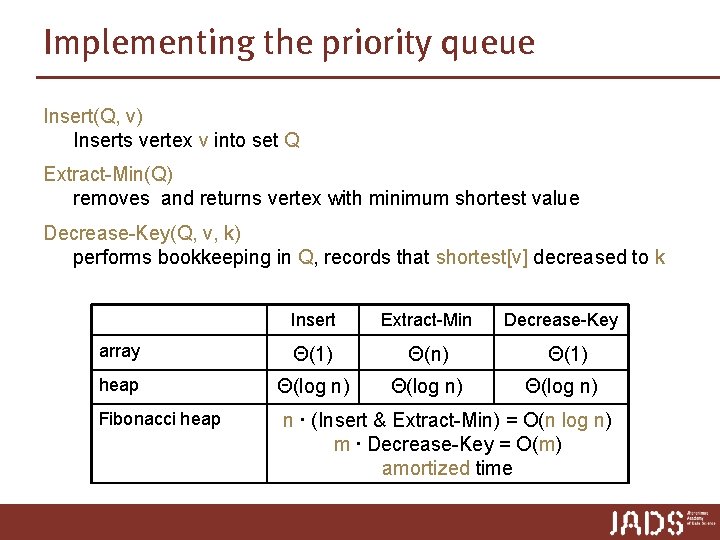
Implementing the priority queue Insert(Q, v) Inserts vertex v into set Q Extract-Min(Q) removes and returns vertex with minimum shortest value Decrease-Key(Q, v, k) performs bookkeeping in Q, records that shortest[v] decreased to k Insert Extract-Min array Θ(1) Θ(n) heap Θ(log n) Fibonacci heap Decrease-Key Θ(1) Θ(log n) n ∙ (Insert & Extract-Min) = O(n log n) m ∙ Decrease-Key = O(m) amortized time

Dijkstra’s algorithm Dijkstra(G, s) 1. Set shortest[v] to ∞ for each v ≠ s, set shortest[s] to 0, and set pred [v] to None for each vertex v 2. Make Q an empty priority queue 3. For each vertex v: A. Call Insert(Q, v) 4. While Q is not empty, do the following A. Call Extract-Min(Q) and set u to hold the returned vertex B. For each vertex v adjacent to u i. Call Relax(u, v) ii. If the call to Relax(u, v) decreased the values of shortest[v], then call Decrease-Key(Q, v) Theorem Dijkstra’s algorithm solves the Single-Source Shortest-Path Problem for graphs with non-negative edge weights in O(V log V + E) time.

P vs NP

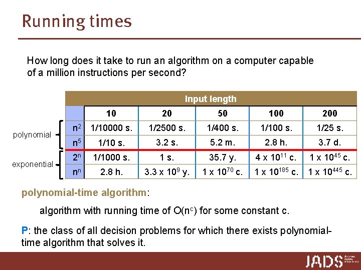
Running times How long does it take to run an algorithm on a computer capable of a million instructions per second? Input length polynomial exponential 10 20 50 100 200 n 2 1/10000 s. 1/2500 s. 1/400 s. 1/100 s. 1/25 s. n 5 1/10 s. 3. 2 s. 5. 2 m. 2. 8 h. 3. 7 d. 2 n 1/1000 s. 1 s. 35. 7 y. 4 x 1011 c. 1 x 1045 c. nn 2. 8 h. 3. 3 x 109 y. 1 x 1070 c. 1 x 10185 c. 1 x 10445 c. polynomial-time algorithm: algorithm with running time of O(nc) for some constant c. P: the class of all decision problems for which there exists polynomialtime algorithm that solves it.

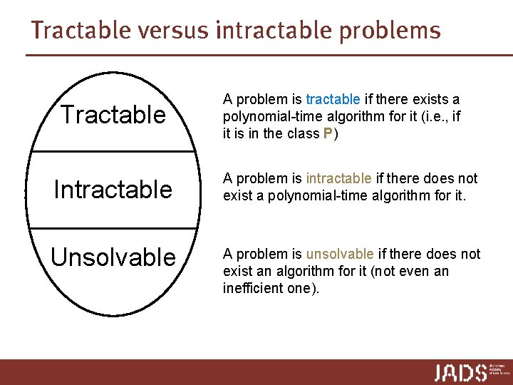
Tractable versus intractable problems Tractable A problem is tractable if there exists a polynomial-time algorithm for it (i. e. , if it is in the class P) Intractable A problem is intractable if there does not exist a polynomial-time algorithm for it. Unsolvable A problem is unsolvable if there does not exist an algorithm for it (not even an inefficient one).

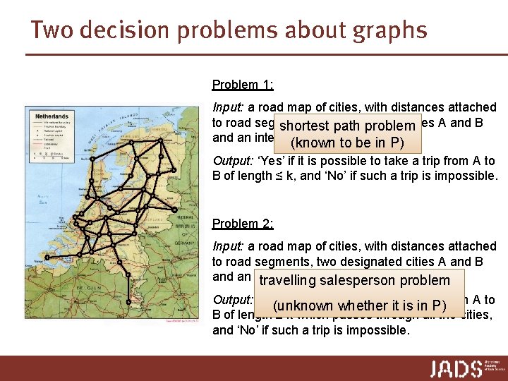
Two decision problems about graphs Problem 1: Input: a road map of cities, with distances attached to road segments, twopath designated cities A and B shortest problem and an integer(known k. to be in P) Output: ‘Yes’ if it is possible to take a trip from A to B of length ≤ k, and ‘No’ if such a trip is impossible. Problem 2: Input: a road map of cities, with distances attached to road segments, two designated cities A and B and an integer k. salesperson problem travelling Output: ‘Yes’ if it is possible to take a trip from A to (unknown whether it is in P) B of length ≤ k which passes through all the cities, and ‘No’ if such a trip is impossible.

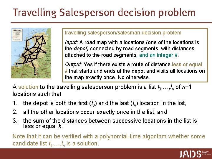
Travelling Salesperson decision problem travelling salesperson/salesman decision problem Input: A road map with n locations (one of the locations is the depot) connected by road segments, with distances attached to the road segments, and an integer k. Output: Yes if there exists a route of distance less or equal k that starts and ends at the depot and visits all locations on the map exactly once. No otherwise. A solution to the travelling salesperson problem is a list l 0, …, ln of n+1 locations such that 1. the depot is both the first (l 0) and the last (ln) location in the list, 2. all the other locations occur exactly once in the list, and 3. the sum of the distances between successive locations in the list is less or equal k. Note that it can be verified with a polynomial-time algorithm whether some candidate list l 0, …, ln is a solution.

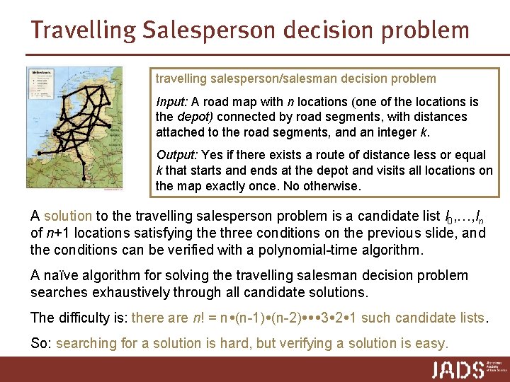
Travelling Salesperson decision problem travelling salesperson/salesman decision problem Input: A road map with n locations (one of the locations is the depot) connected by road segments, with distances attached to the road segments, and an integer k. Output: Yes if there exists a route of distance less or equal k that starts and ends at the depot and visits all locations on the map exactly once. No otherwise. A solution to the travelling salesperson problem is a candidate list l 0, …, ln of n+1 locations satisfying the three conditions on the previous slide, and the conditions can be verified with a polynomial-time algorithm. A naïve algorithm for solving the travelling salesman decision problem searches exhaustively through all candidate solutions. The difficulty is: there are n! = n (n-1) (n-2) 3 2 1 such candidate lists. So: searching for a solution is hard, but verifying a solution is easy.

Problems in NP The travelling salesperson problem has the following characteristics: 1. Given some candidate solution, it can be verified in polynomial time whether it is a correct solution. 2. There are too many candidate solutions to allow an efficient solution that exhaustively searches for a correct solution among the candidate solutions. A candidate solution to a problem will be called a certificate for the problem. NP: the class of all decision problems for which there exists a suitable notion of certificate and a polynomial-time algorithm to verify whether a certificate is an actual solution to the problem. (NP stands for Non-deterministic Polynomial time)

NP-complete problems A problem is in the class NP if there exists a polynomial-time algorithm to verify whether a certificate is an actual solution to the problem. A problem is NP-hard if the existence of a polynomial-time algorithm to solve the problem implies the existence of polynomial-time algorithms for all the other problems in NP. A problem is NP-complete if it is NP-hard and in NP. Theorem: The traveling salesperson problem is NP-complete. If one fails to find an efficient algorithm for a problem then it can be worth investigating whether it is NP-hard. There is a rich algorithmic toolset to deal with NP-hard problems, e. g. , approximation

Recap and preview Today p Single-Source Shortest Path: Dijkstra p Running time depends on priority queue p Perspectives: hard problems Next lecture p Kd-trees