Data Structures Algorithms Lecture Lineartime Sorting The sorting

Data Structures & Algorithms Lecture: Linear-time Sorting

The sorting problem Input: a sequence of n numbers ‹a 0, a 1, …, an-1› Output: a permutation of the input such that ‹ai 0 ≤ … ≤ ain-1› Why do we care so much about sorting? p sorting is used by many applications p (first) step of many algorithms p many techniques can be illustrated by studying sorting

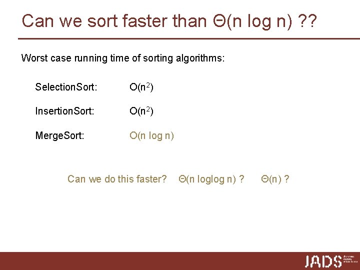
Can we sort faster than Θ(n log n) ? ? Worst case running time of sorting algorithms: Selection. Sort: O(n 2) Insertion. Sort: O(n 2) Merge. Sort: O(n log n) Can we do this faster? Θ(n loglog n) ? Θ(n) ?

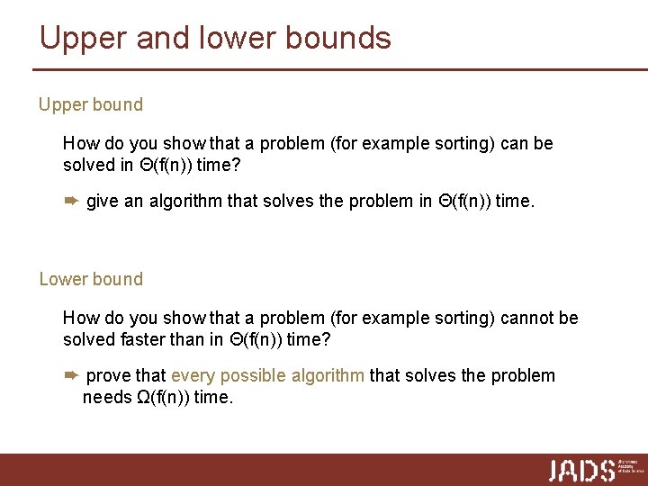
Upper and lower bounds Upper bound How do you show that a problem (for example sorting) can be solved in Θ(f(n)) time? ➨ give an algorithm that solves the problem in Θ(f(n)) time. Lower bound How do you show that a problem (for example sorting) cannot be solved faster than in Θ(f(n)) time? ➨ prove that every possible algorithm that solves the problem needs Ω(f(n)) time.

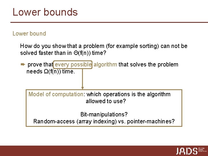
Lower bounds Lower bound How do you show that a problem (for example sorting) can not be solved faster than in Θ(f(n)) time? ➨ prove that every possible algorithm that solves the problem needs Ω(f(n)) time. Model of computation: which operations is the algorithm allowed to use? Bit-manipulations? Random-access (array indexing) vs. pointer-machines?

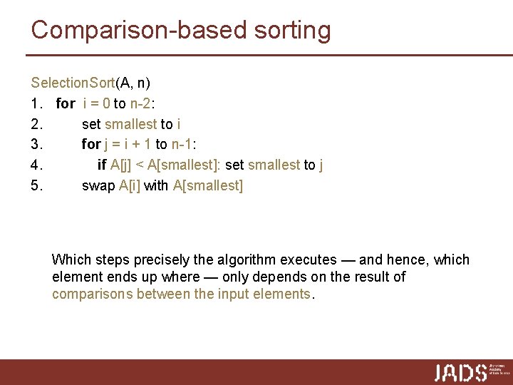
Comparison-based sorting Selection. Sort(A, n) 1. for i = 0 to n-2: 2. set smallest to i 3. for j = i + 1 to n-1: 4. if A[j] < A[smallest]: set smallest to j 5. swap A[i] with A[smallest] Which steps precisely the algorithm executes — and hence, which element ends up where — only depends on the result of comparisons between the input elements.

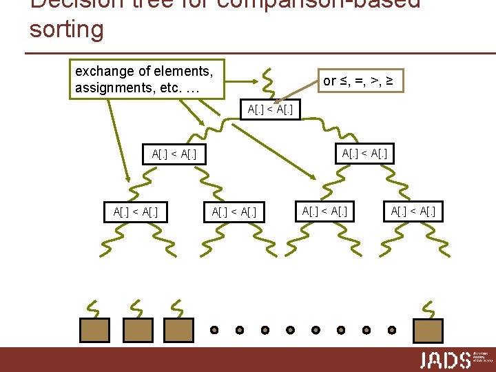
Decision tree for comparison-based sorting exchange of elements, assignments, etc. … or ≤, =, >, ≥ A[. ] < A[. ] A[. ] < A[. ]

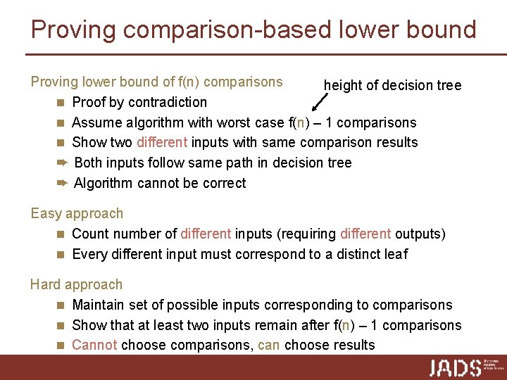
Proving comparison-based lower bound Proving lower bound of f(n) comparisons height of decision tree n Proof by contradiction n Assume algorithm with worst case f(n) – 1 comparisons n Show two different inputs with same comparison results ➨ Both inputs follow same path in decision tree ➨ Algorithm cannot be correct Easy approach n Count number of different inputs (requiring different outputs) n Every different input must correspond to a distinct leaf Hard approach n Maintain set of possible inputs corresponding to comparisons n Show that at least two inputs remain after f(n) – 1 comparisons n Cannot choose comparisons, can choose results

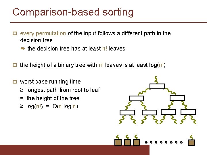
Comparison-based sorting p every permutation of the input follows a different path in the decision tree ➨ the decision tree has at least n! leaves p the height of a binary tree with n! leaves is at least log(n!) p worst case running time ≥ longest path from root to leaf = the height of the tree ≥ log(n!) = Ω(n log n)

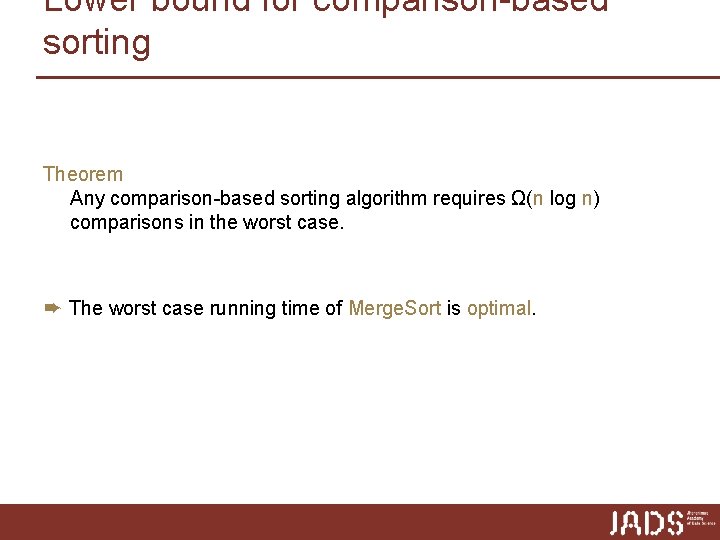
Lower bound for comparison-based sorting Theorem Any comparison-based sorting algorithm requires Ω(n log n) comparisons in the worst case. ➨ The worst case running time of Merge. Sort is optimal.

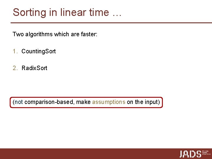
Sorting in linear time … Two algorithms which are faster: 1. Counting. Sort 2. Radix. Sort (not comparison-based, make assumptions on the input)

Counting. Sort Input: array A[0. . n-1] of numbers Assumption: the input elements are integers in the range 0 to k, for some k Main idea: count for every A[i] the number of elements less than A[i] ➨ position of A[i] in the output array Beware of elements that have the same value! position(i) = number of elements less than A[i] in A[0. . n-1] + number of elements equal to A[i] in A[0. . i-1]

Counting. Sort position(i) = number of elements less than A[i] in A[1. . n-1] + number of elements equal to A[i] in A[1. . i-1] 5 3 10 5 4 5 7 7 9 3 10 8 5 3 3 8 3 3 4 5 5 7 7 8 8 9 10 10 numbers < 5 third 5 from left position: (# less than 5) + 2

Counting. Sort position(i) = number of elements less than A[i] in A[1. . n-1] + number of elements equal to A[i] in A[1. . i-1] Lemma If every element A[i] is placed on position(i), then the array is sorted and the sorted order is stable. Numbers with the same value appear in the same order in the output array as they do in the input array.

Counting. Sort C[i] will contain the number of elements ≤ i Counting. Sort(A, k) ► Input: array A[0. . n-1] of integers in the range 0. . k ► Output: array B[0. . n-1] which contains the elements of A, sorted 1. for i = 0 to k do C[i] = 0 2. for j = 0 to A. length-1 do C[A[j]] = C[A[j]] + 1 3. ► C[i] now contains the number of elements equal to i 4. for i = 1 to k do C[i] = C[i] + C[i-1] 5. ► C[i] now contains the number of elements less than or equal to i 6. for j = A. length-1 downto 0 7. do B[C[A[ j ] ] -1] = A[j]; C[A[ j ]] = C[A[ j ]] – 1

Counting. Sort(A, k) ► Input: array A[0. . n-1] of integers in the range 0. . k ► Output: array B[0. . n-1] which contains the elements of A, sorted 1. for i = 0 to k do C[i] = 0 2. for j = 0 to A. length-1 do C[A[j]] = C[A[j]] + 1 3. ► C[i] now contains the number of elements equal to i 4. for i = 1 to k do C[i] = C[i ] + C[i-1] 5. ► C[i] now contains the number of elements less than or equal to i 6. for j = A. length downto 1 7. do B[C[A[ j ] ] -1] = A[j]; C[A[ j ]] = C[A[ j ]] – 1 Correctness lines 6/7: Invariant Inv(j): for j + 1 ≤ i < n: B[position(i)] contains A[i] for 0 ≤ i ≤ k: C[i] = ( # numbers smaller than i ) + ( # numbers equal to i in A[1. . j]) Inv(j) holds before loop is executed, Inv(j – 1) holds afterwards

Counting. Sort: running time Counting. Sort(A, k) ► Input: array A[0. . n-1] of integers in the range 0. . k ► Output: array B[0. . n-1] which contains the elements of A, sorted 1. for i = 0 to k do C[i] = 0 2. for j = 0 to A. length-1 do C[A[j]] = C[A[j]] + 1 3. ► C[i] now contains the number of elements equal to i 4. for i = 1 to k do C[i] = C[i ] + C[i-1] 5. ► C[i] now contains the number of elements less than or equal to i 6. for j = A. length downto 1 7. do B[C[A[ j ] ] -1] = A[j]; C[A[ j ]] = C[A[ j ]] – 1 line 1: ∑ 0≤i≤k Θ(1) = Θ(k) line 2: ∑ 1≤i≤n Θ(1) = Θ(n) line 4: ∑ 0≤i≤k Θ(1) = Θ(k) lines 6/7: ∑ 1≤i≤n Θ(1) = Θ(n) Total: Θ(n+k) ➨ Θ(n) if k = O(n)

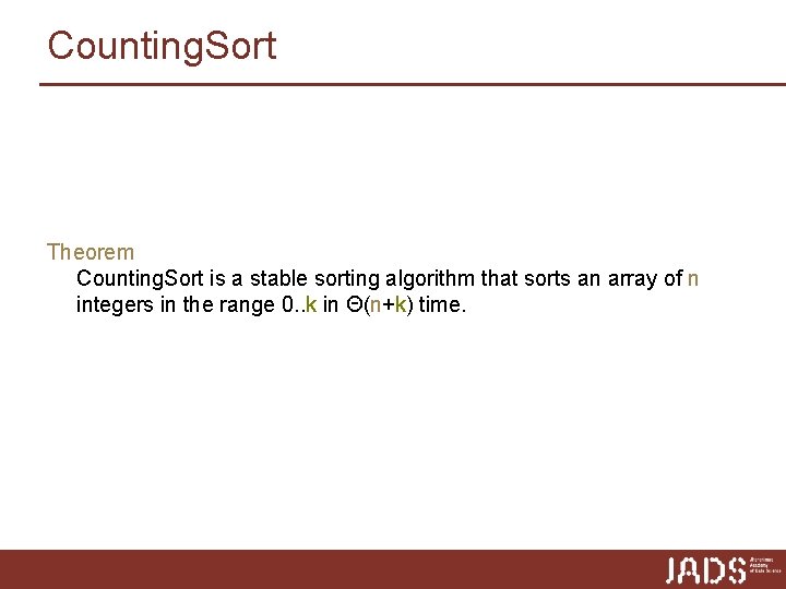
Counting. Sort Theorem Counting. Sort is a stable sorting algorithm that sorts an array of n integers in the range 0. . k in Θ(n+k) time.

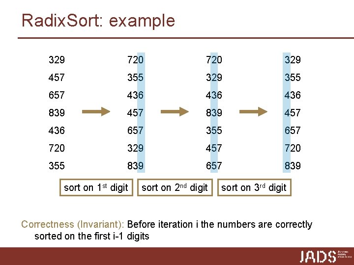
Radix. Sort Input: array A[0. . n-1] of numbers Assumption: the input elements are integers with d digits example (d = 4): 3288, 1193, 9999, 0654, 7243, 4321 dth digit 1 st digit Radix. Sort(A, d) 1. for i = 1 to d 2. do use a stable sort to sort array A on digit i

Radix. Sort: example 329 720 329 457 355 329 355 657 436 436 839 457 436 657 355 657 720 329 457 720 355 839 657 839 sort on 1 st digit sort on 2 nd digit sort on 3 rd digit Correctness (Invariant): Before iteration i the numbers are correctly sorted on the first i-1 digits

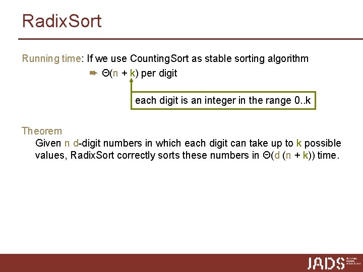
Radix. Sort Running time: If we use Counting. Sort as stable sorting algorithm ➨ Θ(n + k) per digit each digit is an integer in the range 0. . k Theorem Given n d-digit numbers in which each digit can take up to k possible values, Radix. Sort correctly sorts these numbers in Θ(d (n + k)) time.

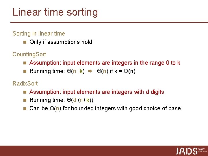
Linear time sorting Sorting in linear time n Only if assumptions hold! Counting. Sort n Assumption: input elements are integers in the range 0 to k n Running time: Θ(n+k) ➨ Θ(n) if k = O(n) Radix. Sort n Assumption: input elements are integers with d digits n Running time: Θ(d (n+k)) n Can be Θ(n) for bounded integers with good choice of base

Recap Today p Models of computation and lower bounds p Sorting is in Ω(n log n) p Linear-time sorting under assumptions n Counting sort n Radix sort p Brief look at Quicksort