Data Structures Algorithms Lecture 3 Sorting Recap Recursion

Data Structures & Algorithms Lecture 3: Sorting

Recap: Recursion

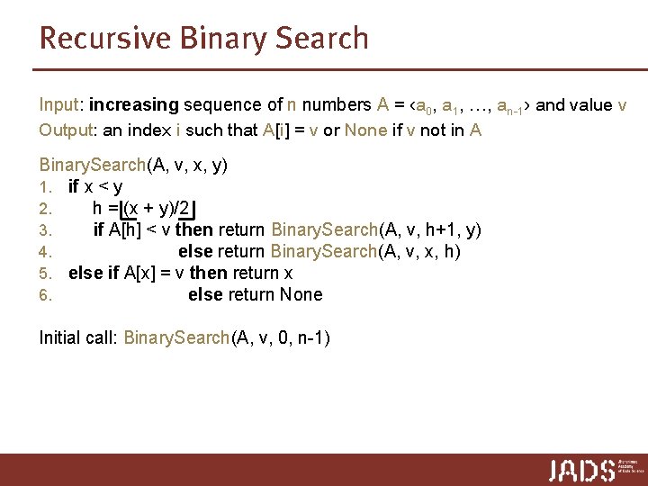
Recursive Binary Search Input: increasing sequence of n numbers A = ‹a 0, a 1, …, an-1› and value v Output: an index i such that A[i] = v or None if v not in A Binary. Search(A, v, x, y) 1. . if x < y 2. h = (x + y)/2 3. if A[h] < v then return Binary. Search(A, v, h+1, y) 4. else return Binary. Search(A, v, x, h) 5. else if A[x] = v then return x 6. else return None Initial call: Binary. Search(A, v, 0, n-1)

Algorithms p A complete description of an algorithm consists of three parts: 1. the algorithm, expressed in whatever way is clearest and most concise 2. a proof of the algorithm’s correctness, for a recursive algorithm: (strong) induction 3. a derivation of the algorithm’s running time for a recursive algorithm: solve a recurrence

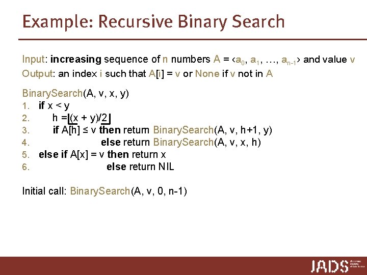
Example: Recursive Binary Search Input: increasing sequence of n numbers A = ‹a 0, a 1, …, an-1› and value v Output: an index i such that A[i] = v or None if v not in A Binary. Search(A, v, x, y) 1. . if x < y 2. h = (x + y)/2 3. if A[h] ≤ v then return Binary. Search(A, v, h+1, y) 4. else return Binary. Search(A, v, x, h) 5. else if A[x] = v then return x 6. else return NIL Initial call: Binary. Search(A, v, 0, n-1)

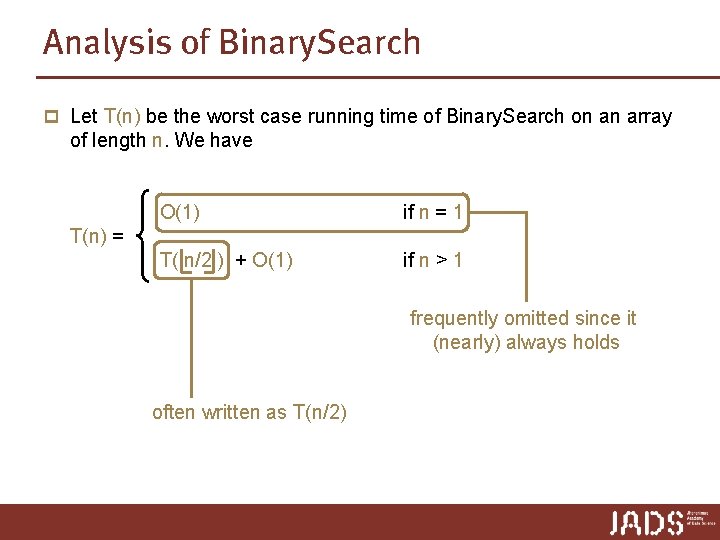
Analysis of Binary. Search p Let T(n) be the worst case running time of Binary. Search on an array of length n. We have O(1) if n = 1 T( n/2 ) + O(1) if n > 1 T(n) = frequently omitted since it (nearly) always holds often written as T(n/2)

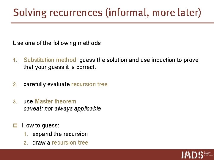
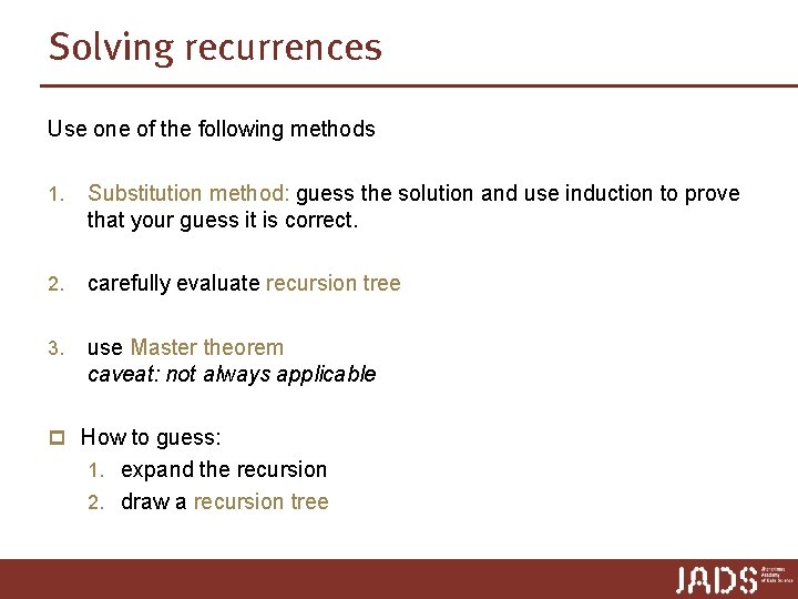
Solving recurrences (informal, more later) Use one of the following methods 1. Substitution method: guess the solution and use induction to prove that your guess it is correct. 2. carefully evaluate recursion tree 3. use Master theorem caveat: not always applicable p How to guess: 1. expand the recursion 2. draw a recursion tree

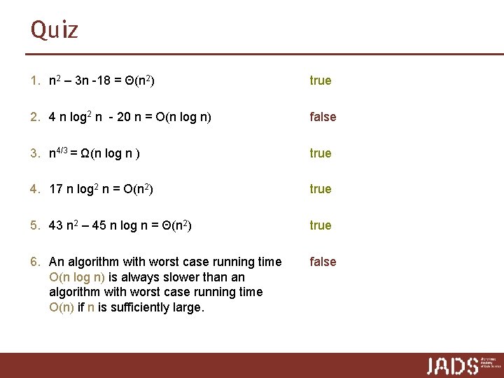
Quiz 1. n 2 – 3 n -18 = Θ(n 2) true 2. 4 n log 2 n - 20 n = O(n log n) false 3. n 4/3 = Ω(n log n ) true 4. 17 n log 2 n = O(n 2) true 5. 43 n 2 – 45 n log n = Θ(n 2) true 6. An algorithm with worst case running time O(n log n) is always slower than an algorithm with worst case running time O(n) if n is sufficiently large. false

Sorting

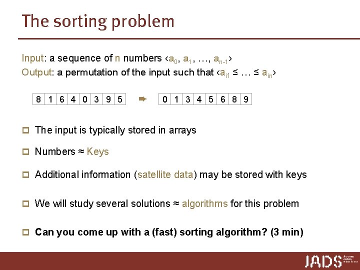
The sorting problem Input: a sequence of n numbers ‹a 0, a 1, …, an-1› Output: a permutation of the input such that ‹ai 1 ≤ … ≤ ain› 8 1 6 4 0 3 9 5 ➨ 0 1 3 4 5 6 8 9 p The input is typically stored in arrays p Numbers ≈ Keys p Additional information (satellite data) may be stored with keys p We will study several solutions ≈ algorithms for this problem p Can you come up with a (fast) sorting algorithm? (3 min)

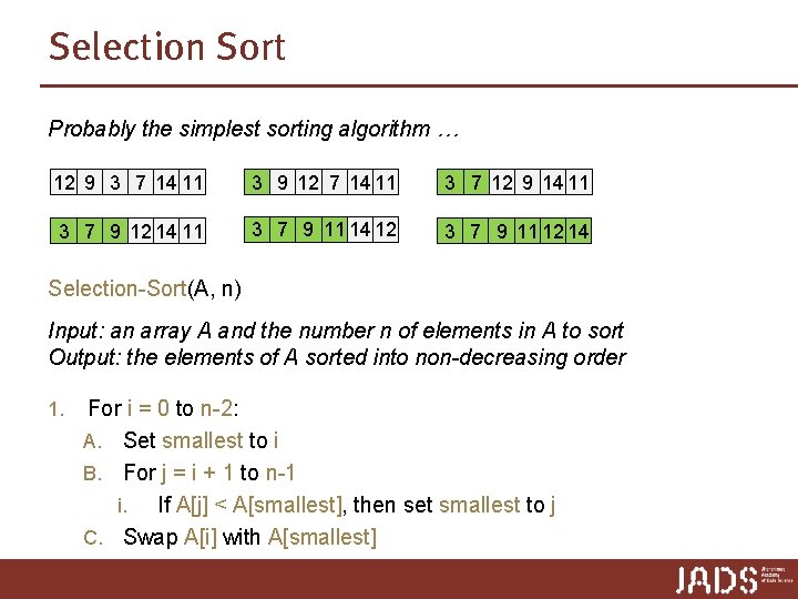
Selection Sort Probably the simplest sorting algorithm … 12 9 3 7 14 11 3 9 12 7 14 11 3 7 12 9 14 11 3 7 9 12 14 11 3 7 9 11 14 12 3 7 9 11 12 14 Selection-Sort(A, n) Input: an array A and the number n of elements in A to sort Output: the elements of A sorted into non-decreasing order 1. For i = 0 to n-2: A. Set smallest to i B. For j = i + 1 to n-1 i. If A[j] < A[smallest], then set smallest to j C. Swap A[i] with A[smallest]

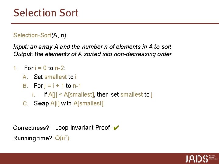
Selection Sort Selection-Sort(A, n) Input: an array A and the number n of elements in A to sort Output: the elements of A sorted into non-decreasing order 1. For i = 0 to n-2: A. Set smallest to i B. For j = i + 1 to n-1 i. If A[j] < A[smallest], then set smallest to j C. Swap A[i] with A[smallest] Correctness? Loop Invariant Proof ✔ Running time? O(n 2)

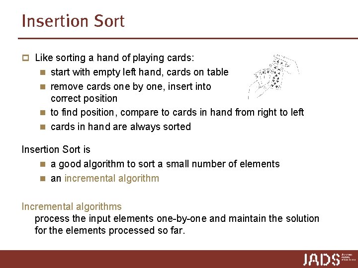
Insertion Sort p Like sorting a hand of playing cards: n start with empty left hand, cards on table n remove cards one by one, insert into correct position n to find position, compare to cards in hand from right to left n cards in hand are always sorted Insertion Sort is n a good algorithm to sort a small number of elements n an incremental algorithm Incremental algorithms process the input elements one-by-one and maintain the solution for the elements processed so far.

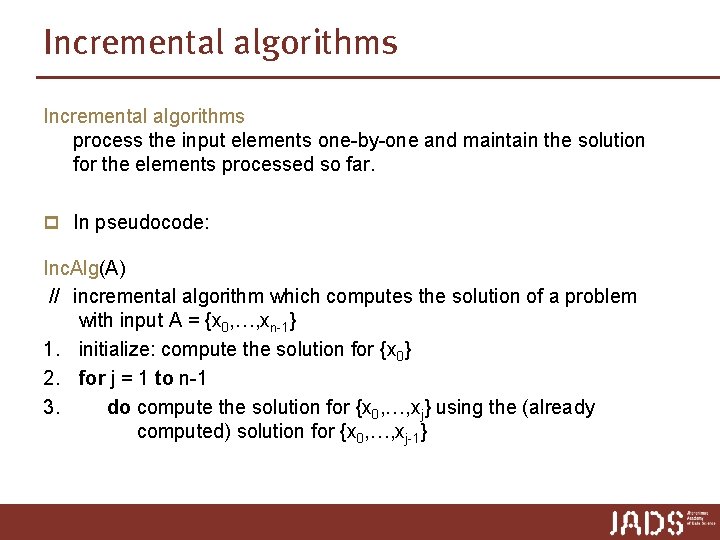
Incremental algorithms process the input elements one-by-one and maintain the solution for the elements processed so far. p In pseudocode: Inc. Alg(A) // incremental algorithm which computes the solution of a problem with input A = {x 0, …, xn-1} 1. initialize: compute the solution for {x 0} 2. for j = 1 to n-1 3. do compute the solution for {x 0, …, xj} using the (already computed) solution for {x 0, …, xj-1}

Insertion Sort Insertion-Sort(A) // incremental algorithm that sorts array A[0: n] in non-decreasing order 1. initialize: sort A[0] 2. for j = 1 to len(A)-1 3. do sort A[0: j+1] using the fact that A[0: j] is already sorted Note: p A[i: j] denotes the array A restricted to the indices ≥ i, and < j (not including j!) p A[: j] is short for A[0: j] p A[i: ] is short for A[i: len(A)]

Insertion Sort Insertion-Sort(A) // incremental algorithm that sorts array A[0: n] in non-decreasing order Insertion Sort is an in place algorithm: 1. initialize: sort A[0] the numbers are rearranged within the 2. for j = 1 to len(A)-1 array with only constant extra space. 3. do key = A[j] 4. i = j -1 5. while i >= 0 and A[i] > key 6. do A[i+1] = A[i] 7. i = i -1 8. A[i +1] = key 0 j 1 3 14 17 28 6 n-1 … For a visualization of sorting algorithms see https: //visualgo. net/en/sorting

Correctness

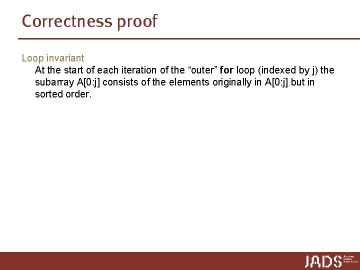
Correctness proof Loop invariant At the start of each iteration of the “outer” for loop (indexed by j) the subarray A[0: j] consists of the elements originally in A[0: j] but in sorted order.

Correctness proof Insertion-Sort(A) 1. initialize: sort A[0] 2. for j = 1 to len(A)-1 3. do key = A[j] 4. i = j -1 5. while i >= 0 and A[i] > key 6. do A[i+1] = A[i] 7. i = i -1 8. A[i +1] = key Loop invariant At the start of each iteration of the “outer” for loop (indexed by j) the subarray A[0: j] consists of the elements originally in A[0: j] but in sorted order. Initialization Just before the first iteration, j = 1 ➨ A[0: j] = [A[0]], which is the element originally in [A[0]], and it is trivially sorted.

Correctness proof Insertion-Sort(A) 1. initialize: sort A[0] 2. for j = 1 to len(A)-1 3. do key = A[j] 4. i = j -1 5. while i >= 0 and A[i] > key 6. do A[i+1] = A[i] 7. i = i -1 8. A[i +1] = key Loop invariant At the start of each iteration of the “outer” for loop (indexed by j) the subarray A[0: j] consists of the elements originally in A[0: j] but in sorted order. Maintenance Strictly speaking need to prove loop invariant for “inner” while loop. Instead, note that body of while loop moves A[j-1], A[j-2], A[j-3], and so on, by one position to the right until proper position of key is found (which has value of A[j]) ➨ invariant maintained.

Correctness proof Insertion-Sort(A) 1. initialize: sort A[0] 2. for j = 1 to len(A)-1 3. do key = A[j] 4. i = j -1 5. while i >= 0 and A[i] > key 6. do A[i+1] = A[i] 7. i = i -1 8. A[i +1] = key Loop invariant At the start of each iteration of the “outer” for loop (indexed by j) the subarray A[0: j] consists of the elements originally in A[0: j] but in sorted order. Termination The outer for loop ends when j = n. Plug n for j in the loop invariant ➨ the subarray A[0: n] consists of the elements originally in A[0: n] in sorted order.

Another sorting algorithm using a different paradigm …

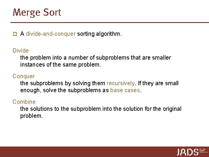
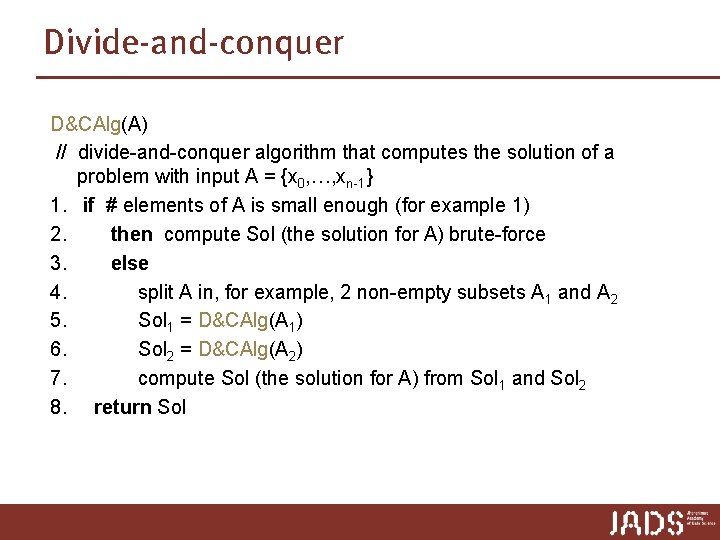
Merge Sort p A divide-and-conquer sorting algorithm. Divide the problem into a number of subproblems that are smaller instances of the same problem. Conquer the subproblems by solving them recursively. If they are small enough, solve the subproblems as base cases. Combine the solutions to the subproblem into the solution for the original problem.

Divide-and-conquer D&CAlg(A) // divide-and-conquer algorithm that computes the solution of a problem with input A = {x 0, …, xn-1} 1. if # elements of A is small enough (for example 1) 2. then compute Sol (the solution for A) brute-force 3. else 4. split A in, for example, 2 non-empty subsets A 1 and A 2 5. Sol 1 = D&CAlg(A 1) 6. Sol 2 = D&CAlg(A 2) 7. compute Sol (the solution for A) from Sol 1 and Sol 2 8. return Sol

Merge Sort Merge-Sort(A) // divide-and-conquer algorithm that sorts array A[0: n] 1. if len(A) == 1 2. then compute Sol (the solution for A) brute-force 3. else 4. split A in 2 non-empty subsets A 1 and A 2 5. Sol 1 = Merge-Sort(A 1) 6. Sol 2 = Merge-Sort(A 2) 7. compute Sol (the solution for A) from Sol 1 en Sol 2

Merge Sort Merge-Sort(A) // divide-and-conquer algorithm that sorts array A[1. . n] 1. if len(A) == 1 2. then skip 3. else 4. n = len(A) ; n 1 = n/2 ; n 2 = n/2 ; copy A[0: n 1] to auxiliary array A 1[0: n 1] copy A[n 1: n] to auxiliary array A 2[n 1: n] 5. Merge-Sort(A 1) 6. Merge-Sort(A 2) 7. Merge(A, A 1, A 2)

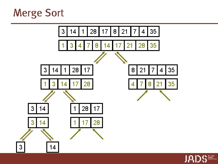
Merge Sort 3 14 1 28 17 8 21 7 4 35 1 3 4 7 8 14 17 21 28 35 3 3 14 1 28 17 8 21 7 4 35 1 3 14 17 28 4 7 8 21 35 3 14 1 28 17 3 14 1 17 28 14

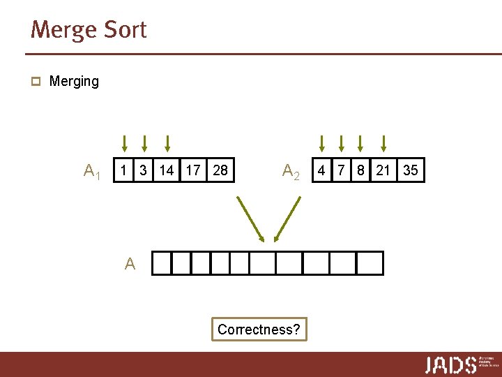
Merge Sort p Merging A 1 1 3 14 17 28 A A 2 4 7 8 21 35 1 3 4 7 8 14 17 21 28 35 Correctness?

Efficiency

Analysis of Insertion Sort Insertion-Sort(A) 1. initialize: sort A[0] 2. for j = 1 to len(A)-1 3. do key = A[j] 4. i = j -1 5. while i >= 0 and A[i] > key 6. do A[i+1] = A[i] 7. i = i -1 8. A[i +1] = key p Get as tight a bound as possible on the worst case running time. ➨ lower and upper bound for worst case running time Upper bound: Analyze worst case number of elementary operations Lower bound: Give “bad” input example

Analysis of Insertion Sort Insertion-Sort(A) 1. initialize: sort A[0] 2. for j = 1 to len(A)-1 3. do key = A[j] 4. i = j -1 5. while i >= 0 and A[i] > key 6. do A[i+1] = A[i] 7. i = i -1 8. A[i +1] = key O(1) worst case: (j-1) ∙ O(1) Upper bound: Let T(n) be the worst case running time of Insertion. Sort on an array of length n. We have T(n) = O(1) + { O(1) + (j-1)∙O(1) + O(1) } = O(j) = O(n 2) Lower bound: Array sorted in de-creasing order ➨ Ω(n 2) The worst case running time of Insertion. Sort is Θ(n 2).

Analysis of Merge Sort Merge-Sort(A) // divide-and-conquer algorithm that sorts array A[0: n] 1. if A. length = 1 2. then skip 3. else 4. n = len(A) ; n 1 = floor(n/2); n 2 = ceil(n/2); 5. copy A[0: n 1] to auxiliary array A 1[0: n 1] 6. copy A[n 1: n] to auxiliary array A 2[0: n 2] 7. Merge-Sort(A 1); Merge-Sort(A 2) 8. Merge(A, A 1, A 2) T( n/2 ) + T( n/2 ) Merge. Sort is a recursive algorithm ➨ running time analysis leads to recursion O(1) O(n) ? ? O(n)

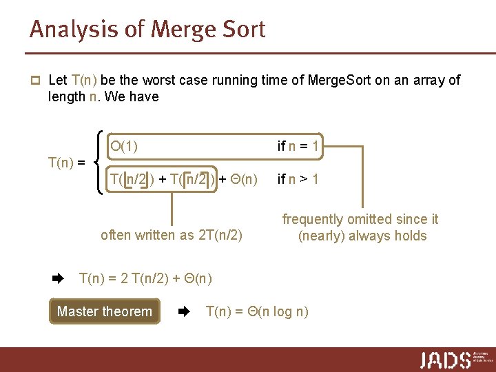
Analysis of Merge Sort p Let T(n) be the worst case running time of Merge. Sort on an array of length n. We have O(1) if n = 1 T( n/2 ) + Θ(n) if n > 1 T(n) = often written as 2 T(n/2) ➨ frequently omitted since it (nearly) always holds T(n) = 2 T(n/2) + Θ(n) Master theorem ➨ T(n) = Θ(n log n)

Solving recurrences

Solving recurrences Use one of the following methods 1. Substitution method: guess the solution and use induction to prove that your guess it is correct. 2. carefully evaluate recursion tree 3. use Master theorem caveat: not always applicable p How to guess: 1. expand the recursion 2. draw a recursion tree

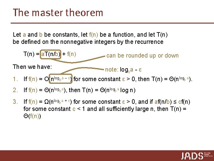
The master theorem Let a and b be constants, let f(n) be a function, and let T(n) be defined on the nonnegative integers by the recurrence T(n) = a. T(n/b) + f(n) Then we have: can be rounded up or down note: logba - ε 1. If f(n) = O(nlogb a – ε) for some constant ε > 0, then T(n) = Θ(nlogb a). 2. If f(n) = Θ(nlogba), then T(n) = Θ(nlogb a log n) 3. If f(n) = Ω(nlogba + ε) for some constant ε > 0, and if af(n/b) ≤ cf(n) for some constant c < 1 and all sufficiently large n, then T(n) = Θ(f(n))

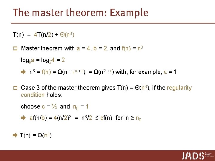
The master theorem: Example T(n) = 4 T(n/2) + Θ(n 3) p Master theorem with a = 4, b = 2, and f(n) = n 3 logba = log 24 = 2 ➨ n 3 = f(n) = Ω(nlogba + ε) = Ω(n 2 + ε) with, for example, ε = 1 p Case 3 of the master theorem gives T(n) = Θ(n 3), if the regularity condition holds. choose c = ½ and n 0 = 1 ➨ af(n/b) = 4(n/2)3 = n 3/2 ≤ cf(n) for n ≥ n 0 ➨ T(n) = Θ(n 3)

Solving recurrences Use one of the following methods 1. Substitution method: guess the solution and use induction to prove that your guess it is correct. 2. carefully evaluate recursion tree 3. use Master theorem caveat: not always applicable p How to guess: 1. expand the recursion 2. draw a recursion tree

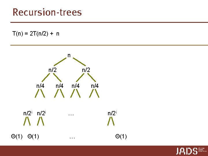
Recursion-trees T(n) = 2 T(n/2) + n n n/2 n/4 n/2 i Θ(1) n/4 n/2 n/4 … … n/4 n/2 i Θ(1)

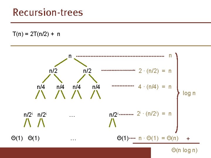
Recursion-trees T(n) = 2 T(n/2) + n n/2 n/4 n/2 i Θ(1) n/4 n/2 n/4 … … 2 ∙ (n/2) = n 4 ∙ (n/4) = n n/4 n/2 i Θ(1) log n 2 i ∙ (n/2 i) = n n ∙ Θ(1) = Θ(n) + Θ(n log n)

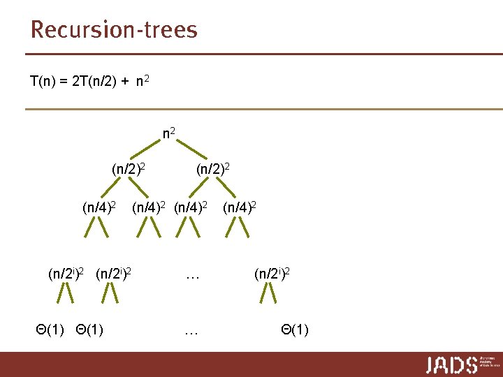
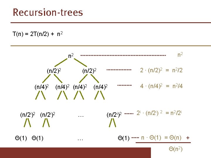
Recursion-trees T(n) = 2 T(n/2) + n 2 (n/2)2 (n/4)2 (n/2 i)2 Θ(1) (n/2)2 (n/4)2 … … (n/4)2 (n/2 i)2 Θ(1)

Recursion-trees T(n) = 2 T(n/2) + n 2 n 2 (n/2)2 (n/4)2 (n/2 i)2 Θ(1) 2 ∙ (n/2)2 = n 2/2 (n/2)2 (n/4)2 … … 4 ∙ (n/4)2 = n 2/4 (n/4)2 (n/2 i)2 Θ(1) 2 i ∙ (n/2 i) 2 = n 2/2 i n ∙ Θ(1) = Θ(n) + Θ(n 2)

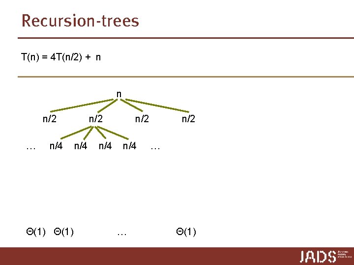
Recursion-trees T(n) = 4 T(n/2) + n n n/2 … n/4 Θ(1) n/2 n/4 … n/2 … Θ(1)

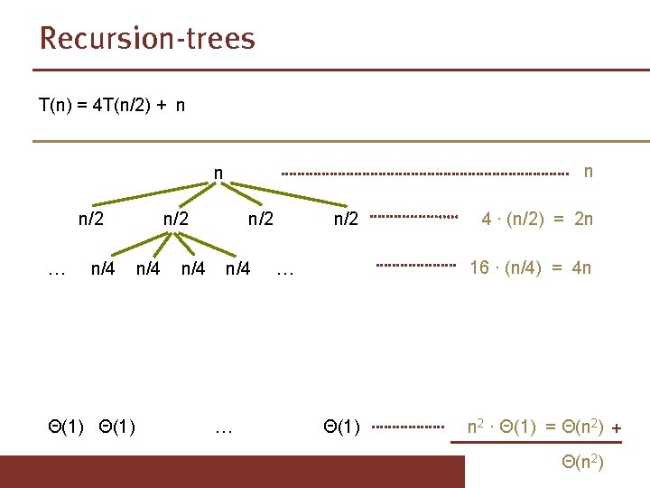
Recursion-trees T(n) = 4 T(n/2) + n n/2 … n/4 Θ(1) n/2 n/4 … n/2 4 ∙ (n/2) = 2 n 16 ∙ (n/4) = 4 n … Θ(1) n 2 ∙ Θ(1) = Θ(n 2) + Θ(n 2)

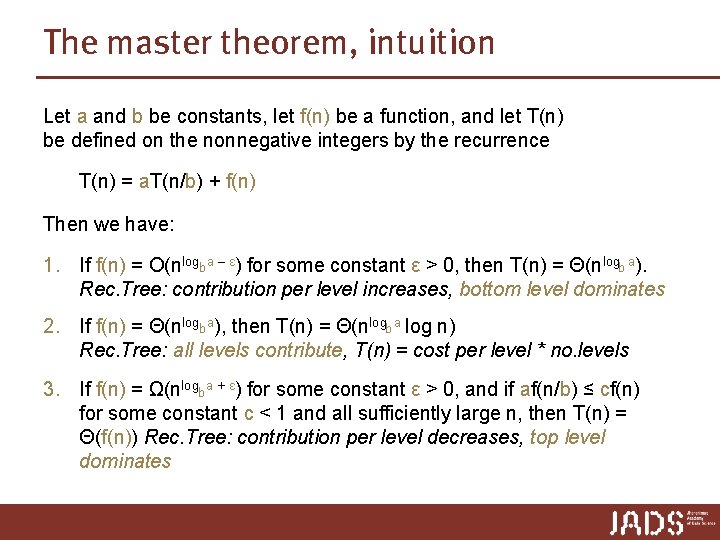
The master theorem, intuition Let a and b be constants, let f(n) be a function, and let T(n) be defined on the nonnegative integers by the recurrence T(n) = a. T(n/b) + f(n) Then we have: 1. If f(n) = O(nlogb a – ε) for some constant ε > 0, then T(n) = Θ(nlogb a). Rec. Tree: contribution per level increases, bottom level dominates 2. If f(n) = Θ(nlogba), then T(n) = Θ(nlogb a log n) Rec. Tree: all levels contribute, T(n) = cost per level * no. levels 3. If f(n) = Ω(nlogba + ε) for some constant ε > 0, and if af(n/b) ≤ cf(n) for some constant c < 1 and all sufficiently large n, then T(n) = Θ(f(n)) Rec. Tree: contribution per level decreases, top level dominates

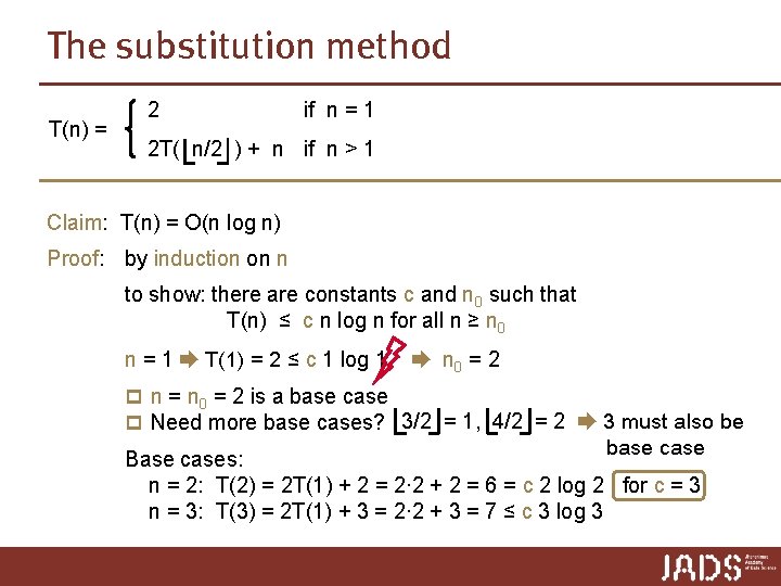
The substitution method T(n) = 2 if n = 1 2 T( n/2 ) + n if n > 1 Claim: T(n) = O(n log n) Proof: by induction on n to show: there are constants c and n 0 such that T(n) ≤ c n log n for all n ≥ n 0 n = 1 ➨ T(1) = 2 ≤ c 1 log 1 ➨ n 0 = 2 p n = n 0 = 2 is a base case p Need more base cases? 3/2 = 1, 4/2 = 2 ➨ 3 must also be base case Base cases: n = 2: T(2) = 2 T(1) + 2 = 2∙ 2 + 2 = 6 = c 2 log 2 for c = 3 n = 3: T(3) = 2 T(1) + 3 = 2∙ 2 + 3 = 7 ≤ c 3 log 3

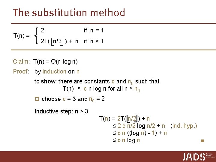
The substitution method T(n) = 2 if n = 1 2 T( n/2 ) + n if n > 1 Claim: T(n) = O(n log n) Proof: by induction on n to show: there are constants c and n 0 such that T(n) ≤ c n log n for all n ≥ n 0 p choose c = 3 and n 0 = 2 Inductive step: n > 3 T(n) = 2 T( n/2 ) + n ≤ 2 c n/2 log n/2 + n (ind. hyp. ) ≤ c n ((log n) - 1) + n ≤ c n log n ■

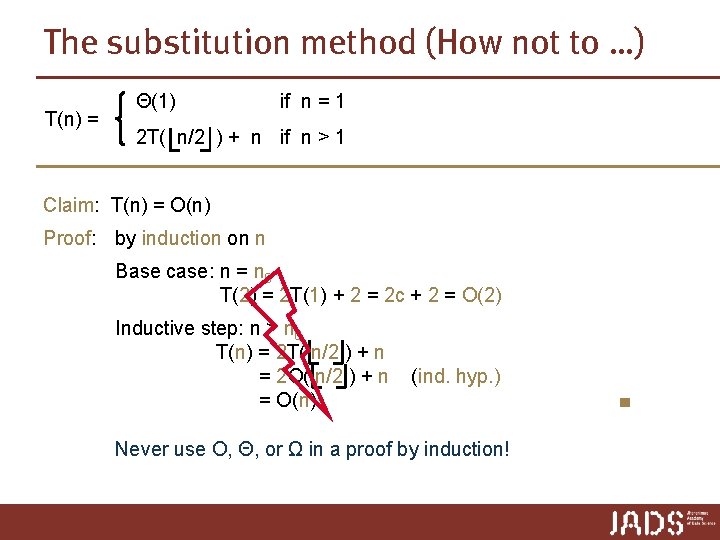
The substitution method (How not to …) T(n) = Θ(1) if n = 1 2 T( n/2 ) + n if n > 1 Claim: T(n) = O(n) Proof: by induction on n Base case: n = n 0 T(2) = 2 T(1) + 2 = 2 c + 2 = O(2) Inductive step: n > n 0 T(n) = 2 T( n/2 ) + n = 2 O( n/2 ) + n = O(n) (ind. hyp. ) Never use O, Θ, or Ω in a proof by induction! ■

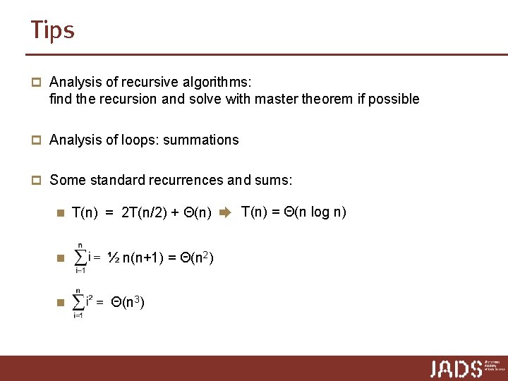
Tips p Analysis of recursive algorithms: find the recursion and solve with master theorem if possible p Analysis of loops: summations p Some standard recurrences and sums: n T(n) = 2 T(n/2) + Θ(n) ➨ T(n) = Θ(n log n) n ½ n(n+1) = Θ(n 2) n Θ(n 3)

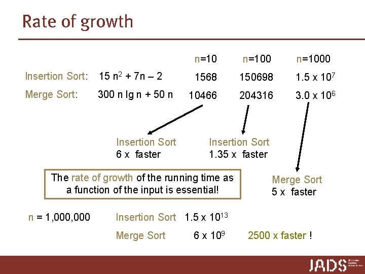
Rate of growth Insertion Sort: 15 n 2 + 7 n – 2 Merge Sort: 300 n lg n + 50 n Insertion Sort 6 x faster n=1000 1568 150698 1. 5 x 107 10466 204316 3. 0 x 106 Insertion Sort 1. 35 x faster The rate of growth of the running time as a function of the input is essential! n = 1, 000 Merge Sort 5 x faster Insertion Sort 1. 5 x 1013 Merge Sort 6 x 109 2500 x faster !

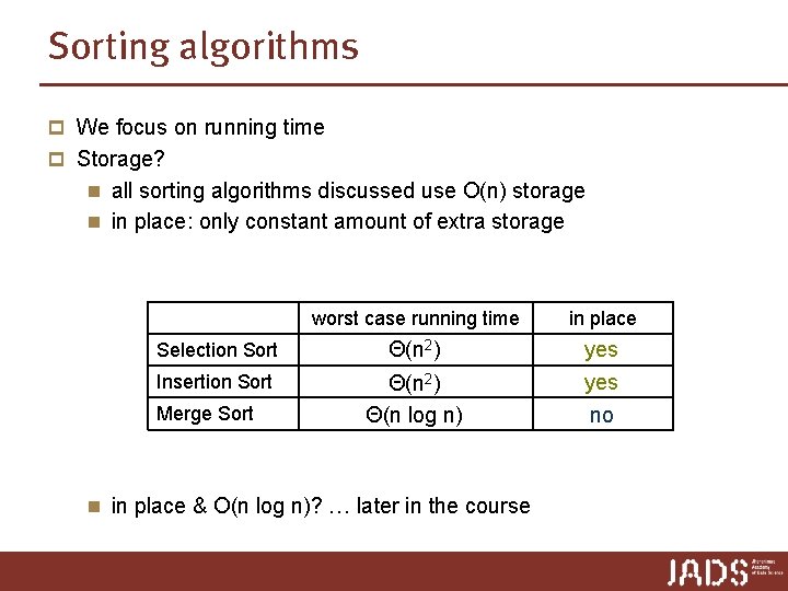
Sorting algorithms p We focus on running time p Storage? n all sorting algorithms discussed use O(n) storage n in place: only constant amount of extra storage worst case running time in place Selection Sort Θ(n 2) yes Insertion Sort Θ(n 2) Θ(n log n) yes no Merge Sort n in place & O(n log n)? … later in the course

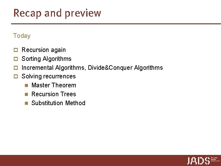
Recap and preview Today p Recursion again p Sorting Algorithms p Incremental Algorithms, Divide&Conquer Algorithms p Solving recurrences n Master Theorem n Recursion Trees n Substitution Method