Data Structures Algorithms Lecture 2 Efficiency analysis binary

Data Structures & Algorithms Lecture 2: Efficiency analysis, binary search & recursion

Overview p Efficiency analysis p Recap/Exercise: sums, induction p Binary search, recursion p Outlook: solving recurrences

Announcements: assignments p Make sure to have an early start on the assignment, let me know about any issues in the group (groups can change) p Did you find a group? p After the deadline the solutions will be discussed in class. They will not be posted on the course page. There are however many exercises with solutions on the course page. p Let us know in case you need any further materials

Recap: Algorithms p A complete description of an algorithm consists of three parts: 1. the algorithm, expressed in whatever way is clearest and most concise 2. a proof of the algorithm’s correctness 3. a derivation of the algorithm’s running time

Efficiency

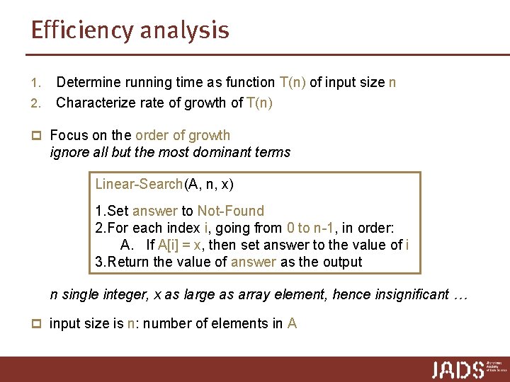
Efficiency analysis 1. 2. Determine running time as function T(n) of input size n Characterize rate of growth of T(n) p Focus on the order of growth ignore all but the most dominant terms Linear-Search(A, n, x) 1. Set answer to Not-Found 2. For each index i, going from 0 to n-1, in order: A. If A[i] = x, then set answer to the value of i 3. Return the value of answer as the output n single integer, x as large as array element, hence insignificant … p input size is n: number of elements in A

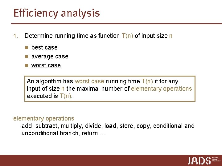
Efficiency analysis 1. Determine running time as function T(n) of input size n n best case n average case n worst case An algorithm has worst case running time T(n) if for any input of size n the maximal number of elementary operations executed is T(n). elementary operations add, subtract, multiply, divide, load, store, copy, conditional and unconditional branch, return …

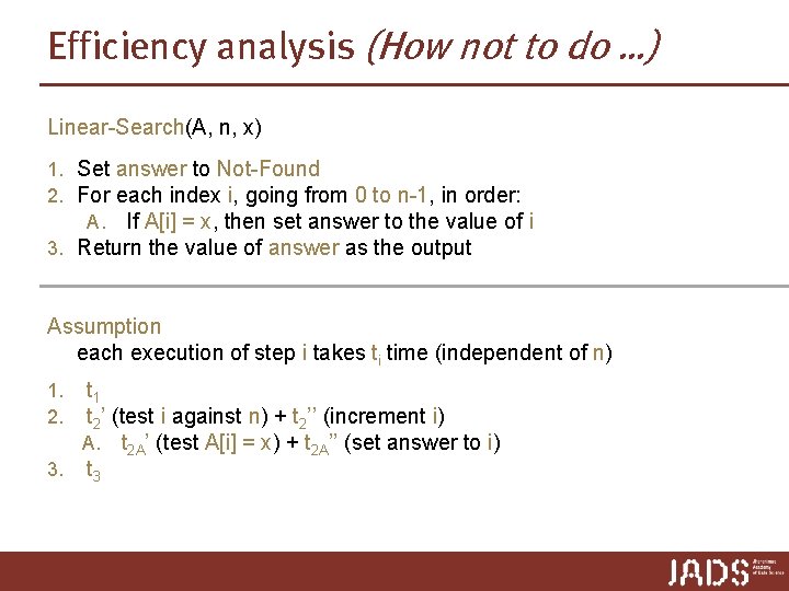
Efficiency analysis (How not to do …) Linear-Search(A, n, x) 1. Set answer to Not-Found 2. For each index i, going from 0 to n-1, in order: A. If A[i] = x, then set answer to the value of i 3. Return the value of answer as the output Assumption each execution of step i takes ti time (independent of n) t 1 t 2’ (test i against n) + t 2’’ (increment i) A. t 2 A’ (test A[i] = x) + t 2 A’’ (set answer to i) 3. t 3 1. 2.

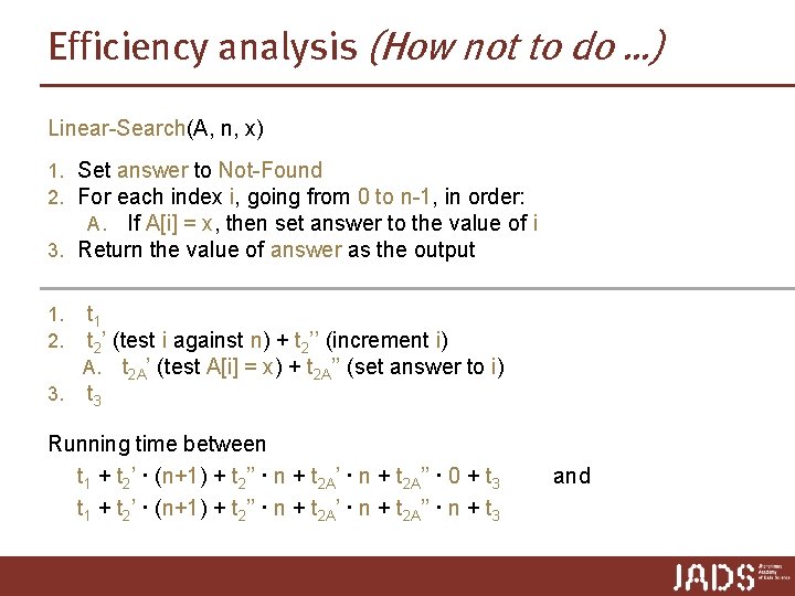
Efficiency analysis (How not to do …) Linear-Search(A, n, x) 1. Set answer to Not-Found 2. For each index i, going from 0 to n-1, in order: A. If A[i] = x, then set answer to the value of i 3. Return the value of answer as the output t 1 t 2’ (test i against n) + t 2’’ (increment i) A. t 2 A’ (test A[i] = x) + t 2 A’’ (set answer to i) 3. t 3 1. 2. Running time between t 1 + t 2’ ∙ (n+1) + t 2’’ ∙ n + t 2 A’’ ∙ 0 + t 3 t 1 + t 2’ ∙ (n+1) + t 2’’ ∙ n + t 2 A’’ ∙ n + t 3 and

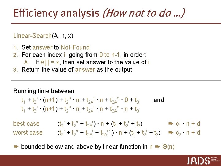
Efficiency analysis (How not to do …) Linear-Search(A, n, x) 1. Set answer to Not-Found 2. For each index i, going from 0 to n-1, in order: A. If A[i] = x, then set answer to the value of i 3. Return the value of answer as the output Running time between t 1 + t 2’ ∙ (n+1) + t 2’’ ∙ n + t 2 A’’ ∙ 0 + t 3 t 1 + t 2’ ∙ (n+1) + t 2’’ ∙ n + t 2 A’’ ∙ n + t 3 best case worst case and (t 2’ + t 2’’ + t 2 A’) ∙ n + (t 1 + t 2’ + t 3) (t 2’ + t 2’’ + t 2 A’’ ) ∙ n + (t 1 + t 2’ + t 3) ➨ c 1 ∙ n + d ➨ c 2 ∙ n + d ➨ bounded below and above by linear function in n ➨ Θ(n)

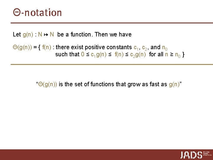
Θ-notation Let g(n) : N ↦ N be a function. Then we have Θ(g(n)) = { f(n) : there exist positive constants c 1, c 2, and n 0 such that 0 ≤ c 1 g(n) ≤ f(n) ≤ c 2 g(n) for all n ≥ n 0 } “Θ(g(n)) is the set of functions that grow as fast as g(n)”

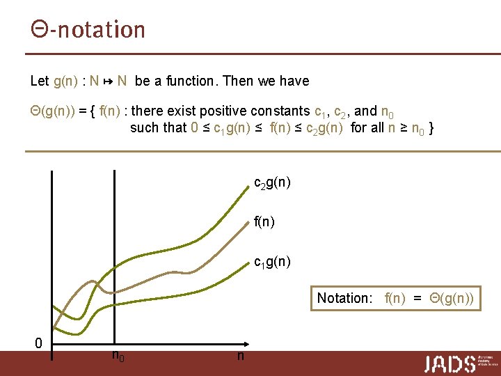
Θ-notation Let g(n) : N ↦ N be a function. Then we have Θ(g(n)) = { f(n) : there exist positive constants c 1, c 2, and n 0 such that 0 ≤ c 1 g(n) ≤ f(n) ≤ c 2 g(n) for all n ≥ n 0 } c 2 g(n) f(n) c 1 g(n) Notation: f(n) = Θ(g(n)) 0 n

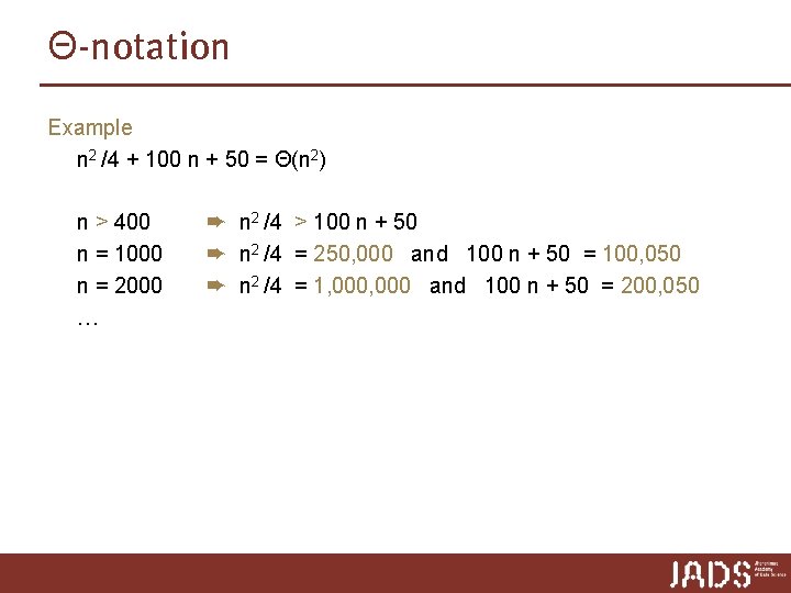
Θ-notation Example n 2 /4 + 100 n + 50 = Θ(n 2) n > 400 n = 1000 n = 2000 … ➨ n 2 /4 > 100 n + 50 ➨ n 2 /4 = 250, 000 and 100 n + 50 = 100, 050 ➨ n 2 /4 = 1, 000 and 100 n + 50 = 200, 050

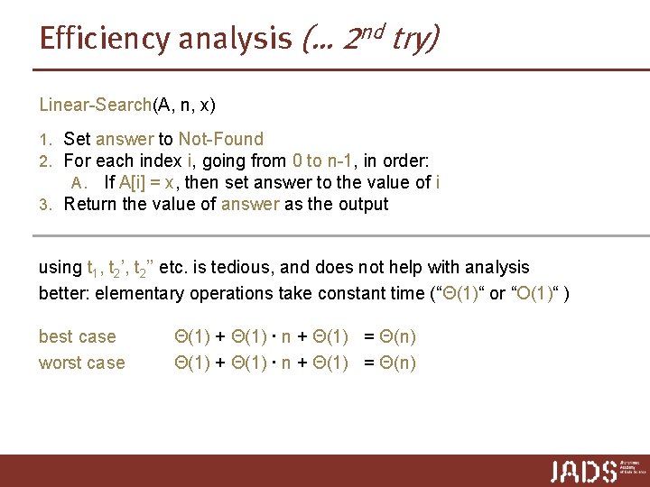
Efficiency analysis (… 2 nd try) Linear-Search(A, n, x) 1. Set answer to Not-Found 2. For each index i, going from 0 to n-1, in order: A. If A[i] = x, then set answer to the value of i 3. Return the value of answer as the output using t 1, t 2’’ etc. is tedious, and does not help with analysis better: elementary operations take constant time (“Θ(1)“ or “O(1)“ ) best case worst case Θ(1) + Θ(1) ∙ n + Θ(1) = Θ(n)

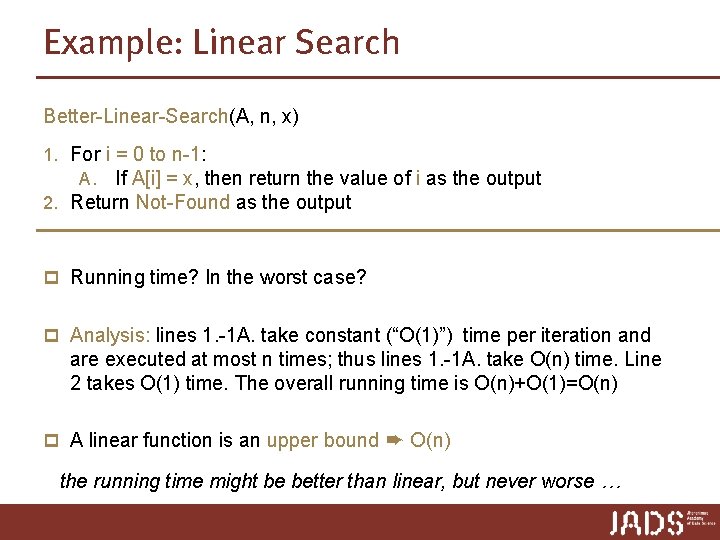
Example: Linear Search Better-Linear-Search(A, n, x) 1. For i = 0 to n-1: A. If A[i] = x, then return the value of i as the output 2. Return Not-Found as the output p Running time? In the worst case? p Analysis: lines 1. -1 A. take constant (“O(1)”) time per iteration and are executed at most n times; thus lines 1. -1 A. take O(n) time. Line 2 takes O(1) time. The overall running time is O(n)+O(1)=O(n) p A linear function is an upper bound ➨ O(n) the running time might be better than linear, but never worse …

O-notation Let g(n) : N ↦ N be a function. Then we have O(g(n)) = { f(n) : there exist positive constants c and n 0 such that 0 ≤ f(n) ≤ cg(n) for all n ≥ n 0 } “O(g(n)) is the set of functions that grow at most as fast as g(n)”

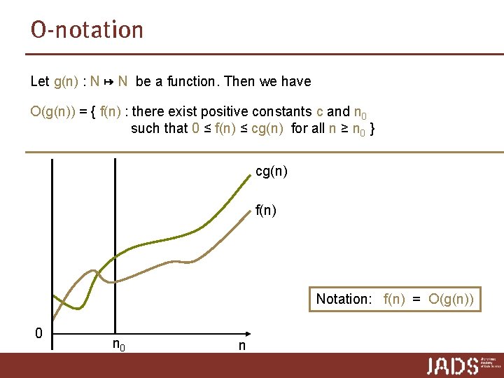
O-notation Let g(n) : N ↦ N be a function. Then we have O(g(n)) = { f(n) : there exist positive constants c and n 0 such that 0 ≤ f(n) ≤ cg(n) for all n ≥ n 0 } cg(n) f(n) Notation: f(n) = O(g(n)) 0 n

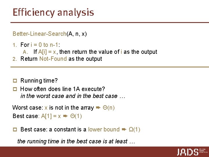
Efficiency analysis Better-Linear-Search(A, n, x) 1. For i = 0 to n-1: A. If A[i] = x, then return the value of i as the output 2. Return Not-Found as the output p Running time? p How often does line 1 A execute? in the worst case and in the best case … Worst case: x is not in the array ➨ Θ(n) Best case: A[1] = x ➨ Θ(1) p Best case: a constant is a lower bound ➨ Ω(1) the running time in the best case is at least …

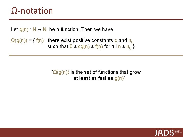
Ω-notation Let g(n) : N ↦ N be a function. Then we have Ω(g(n)) = { f(n) : there exist positive constants c and n 0 such that 0 ≤ cg(n) ≤ f(n) for all n ≥ n 0 } “Ω(g(n)) is the set of functions that grow at least as fast as g(n)”

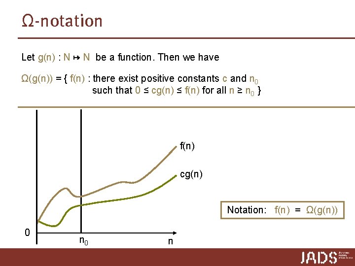
Ω-notation Let g(n) : N ↦ N be a function. Then we have Ω(g(n)) = { f(n) : there exist positive constants c and n 0 such that 0 ≤ cg(n) ≤ f(n) for all n ≥ n 0 } f(n) cg(n) Notation: f(n) = Ω(g(n)) 0 n

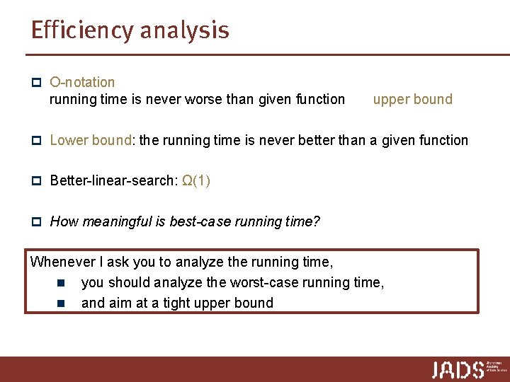
Efficiency analysis p O-notation running time is never worse than given function upper bound p Lower bound: the running time is never better than a given function p Better-linear-search: Ω(1) p How meaningful is best-case running time? Whenever I ask you to analyze the running time, n you should analyze the worst-case running time, n and aim at a tight upper bound

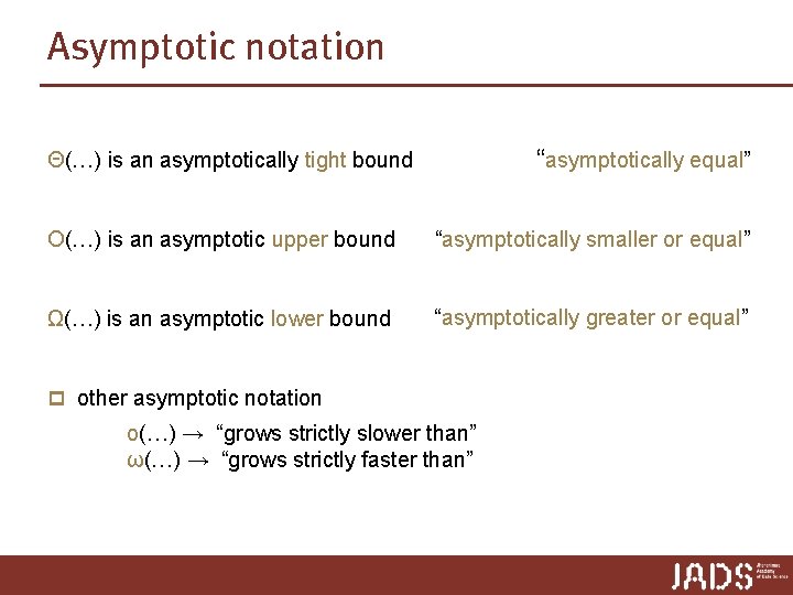
Asymptotic notation “asymptotically equal” Θ(…) is an asymptotically tight bound O(…) is an asymptotic upper bound “asymptotically smaller or equal” Ω(…) is an asymptotic lower bound “asymptotically greater or equal” p other asymptotic notation o(…) → “grows strictly slower than” ω(…) → “grows strictly faster than”

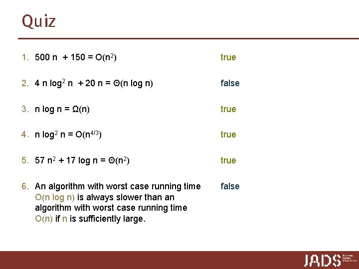
Quiz 1. 500 n + 150 = O(n 2) true 2. 4 n log 2 n + 20 n = Θ(n log n) false 3. n log n = Ω(n) true 4. n log 2 n = O(n 4/3) true 5. 57 n 2 + 17 log n = Θ(n 2) true 6. An algorithm with worst case running time O(n log n) is always slower than an algorithm with worst case running time O(n) if n is sufficiently large. false

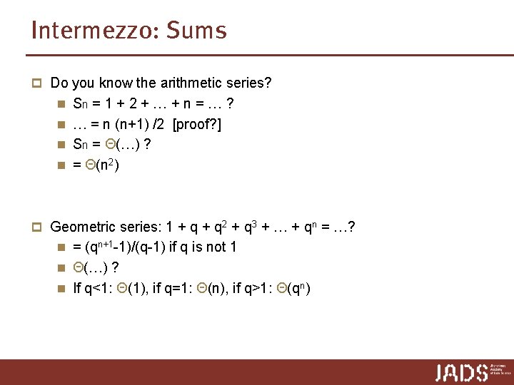
Intermezzo: Sums p Do you know the arithmetic series? n Sn = 1 + 2 + … + n = … ? n … = n (n+1) /2 [proof? ] n Sn = Θ(…) ? n = Θ(n 2) p Geometric series: 1 + q 2 + q 3 + … + qn = …? n = (qn+1 -1)/(q-1) if q is not 1 n Θ(…) ? n If q<1: Θ(1), if q=1: Θ(n), if q>1: Θ(qn)

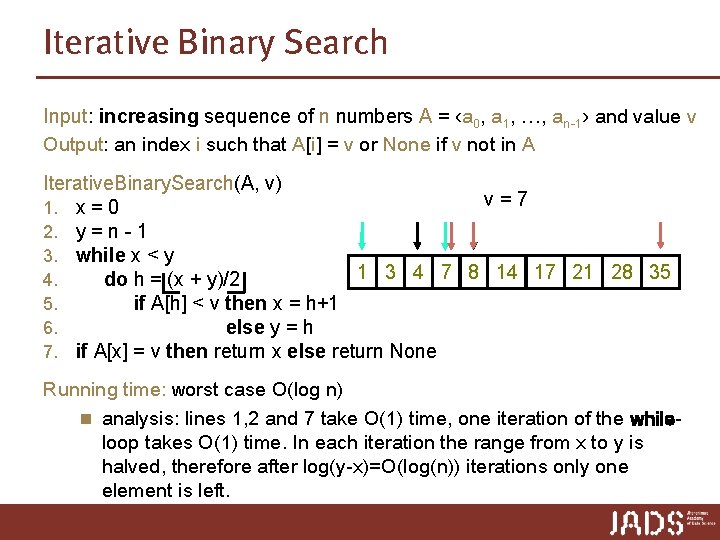
Iterative Binary Search Input: increasing sequence of n numbers A = ‹a 0, a 1, …, an-1› and value v Output: an index i such that A[i] = v or None if v not in A Iterative. Binary. Search(A, v) v=7 1. x = 0 2. y = n - 1 3. while x < y 1 3 4 7 8 14 17 21 28 35 4. do h = (x + y)/2 5. do if A[h] < v then x = h+1 6. else y = h 7. if A[x] = v then return x else return None Running time: worst case O(log n) n analysis: lines 1, 2 and 7 take O(1) time, one iteration of the whileloop takes O(1) time. In each iteration the range from x to y is halved, therefore after log(y-x)=O(log(n)) iterations only one element is left. :

RECURSIVE ALGORITHMS

Recursion p “Recursion“: defining something in terms of itself: n n A directory is a collection of files and directories. Words in dictionaries are defined in terms of other words.

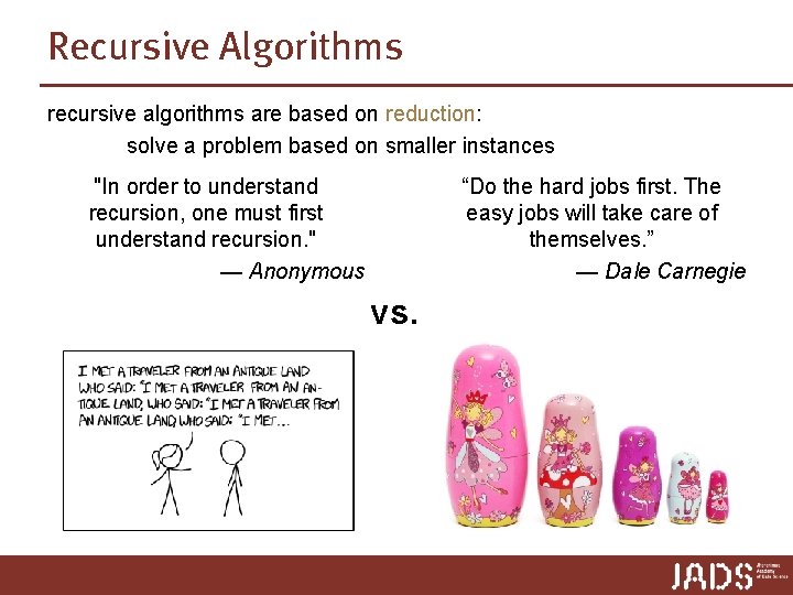
Recursive Algorithms recursive algorithms are based on reduction: solve a problem based on smaller instances "In order to understand recursion, one must first understand recursion. " — Anonymous “Do the hard jobs first. The easy jobs will take care of themselves. ” — Dale Carnegie vs.

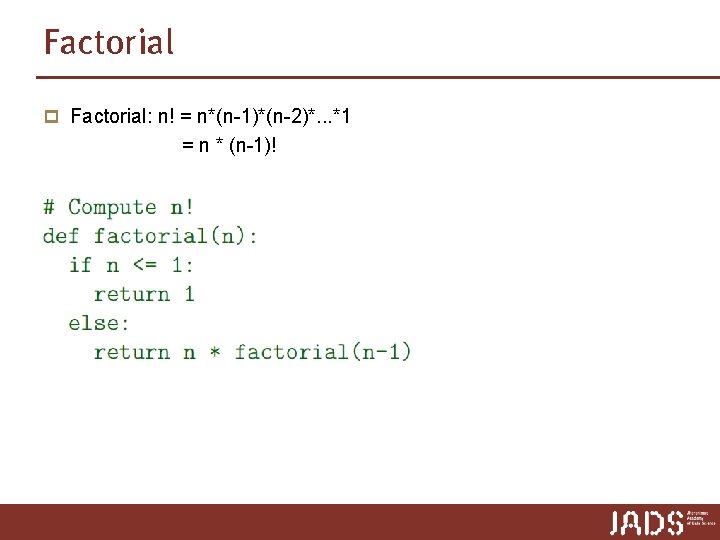
Factorial p Factorial: n! = n*(n-1)*(n-2)*. . . *1 = n * (n-1)!

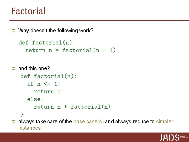
Factorial p Why doesn’t the following work? p and this one? p always take care of the base case(s) and always reduce to simpler instances

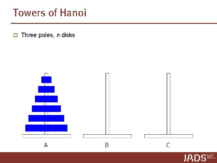
Towers of Hanoi p Three poles, n disks

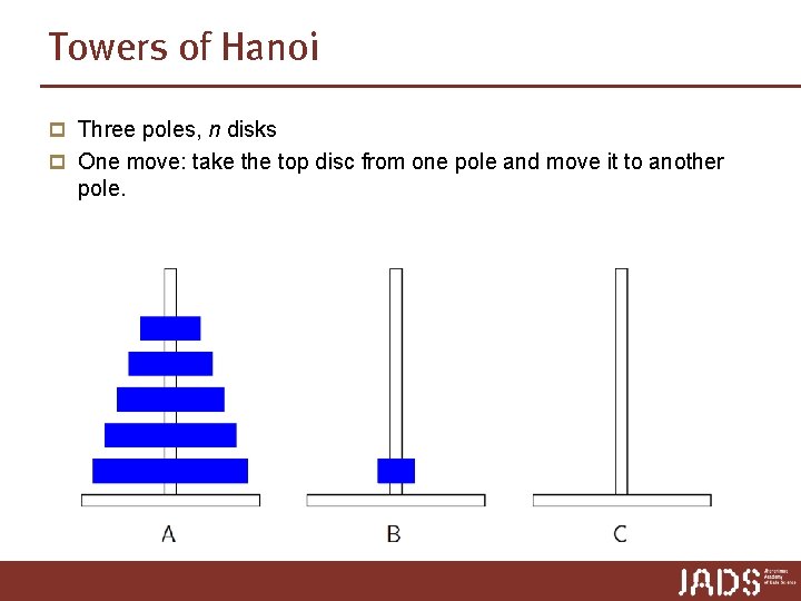
Towers of Hanoi p Three poles, n disks p One move: take the top disc from one pole and move it to another pole.

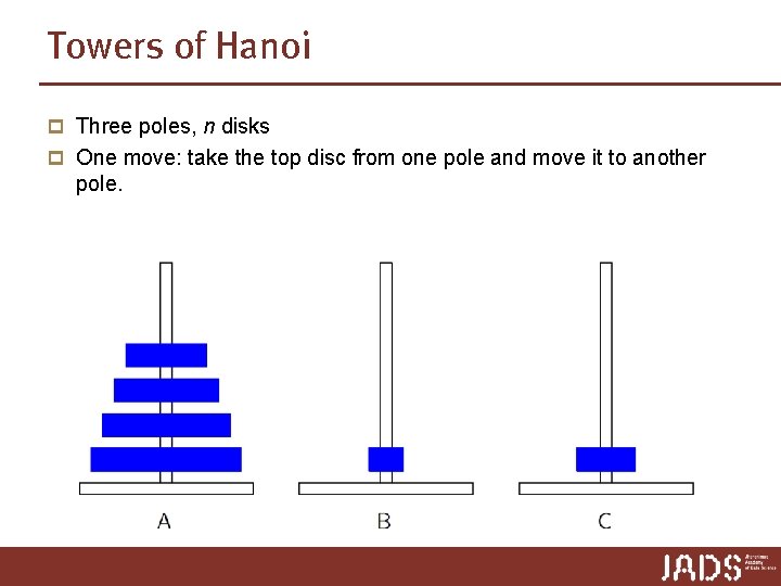
Towers of Hanoi p Three poles, n disks p One move: take the top disc from one pole and move it to another pole.

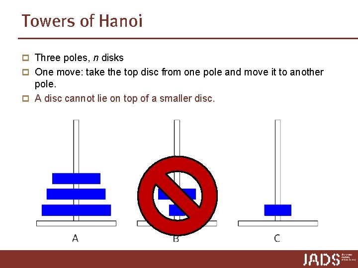
Towers of Hanoi p Three poles, n disks p One move: take the top disc from one pole and move it to another pole. p A disc cannot lie on top of a smaller disc.

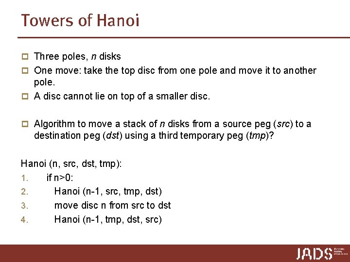
Towers of Hanoi p Three poles, n disks p One move: take the top disc from one pole and move it to another pole. p A disc cannot lie on top of a smaller disc. p Algorithm to move a stack of n disks from a source peg (src) to a destination peg (dst) using a third temporary peg (tmp)? Hanoi (n, src, dst, tmp): 1. if n>0: 2. Hanoi (n-1, src, tmp, dst) 3. move disc n from src to dst 4. Hanoi (n-1, tmp, dst, src)

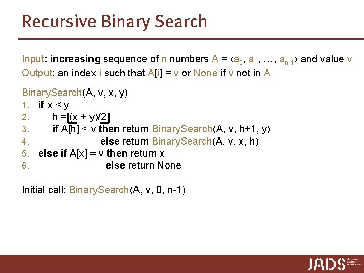
Recursive Binary Search Input: increasing sequence of n numbers A = ‹a 0, a 1, …, an-1› and value v Output: an index i such that A[i] = v or None if v not in A Binary. Search(A, v, x, y) 1. . if x < y 2. h = (x + y)/2 3. if A[h] < v then return Binary. Search(A, v, h+1, y) 4. else return Binary. Search(A, v, x, h) 5. else if A[x] = v then return x 6. else return None Initial call: Binary. Search(A, v, 0, n-1)

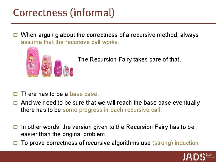
Correctness (informal) p When arguing about the correctness of a recursive method, always assume that the recursive call works. The Recursion Fairy takes care of that. p There has to be a base case. p And we need to be sure that we will reach the base case eventually there has to be some progress in each recursive call. p In other words, the version given to the Recursion Fairy has to be easier than the original problem. p To prove correctness of recursive algorithms use (strong) induction

Algorithms p A complete description of an algorithm consists of three parts: 1. the algorithm, expressed in whatever way is clearest and most concise 2. a proof of the algorithm’s correctness 3. a derivation of the algorithm’s running time ? ? ? We will discuss the analysis of the running time of recursive algorithms in more detail in the next lecture … but here is a preview

Solving recurrences

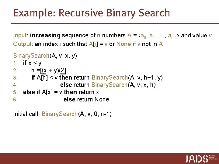
Example: Recursive Binary Search Input: increasing sequence of n numbers A = ‹a 0, a 1, …, an-1› and value v Output: an index i such that A[i] = v or None if v not in A Binary. Search(A, v, x, y) 1. . if x < y 2. h = (x + y)/2 3. if A[h] < v then return Binary. Search(A, v, h+1, y) 4. else return Binary. Search(A, v, x, h) 5. else if A[x] = v then return x 6. else return None Initial call: Binary. Search(A, v, 0, n-1)

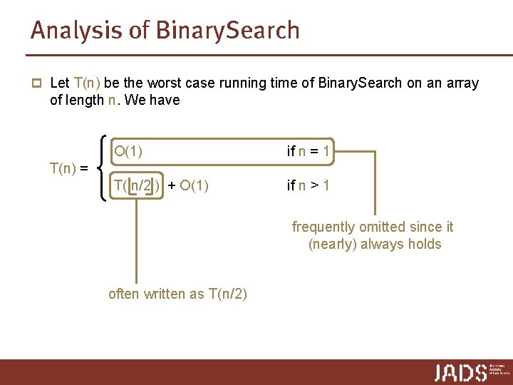
Analysis of Binary. Search p Let T(n) be the worst case running time of Binary. Search on an array of length n. We have O(1) if n = 1 T( n/2 ) + O(1) if n > 1 T(n) = frequently omitted since it (nearly) always holds often written as T(n/2)

Solving recurrences (more in next lecture) Use one of the following methods 1. Substitution method: guess the solution and use induction to prove that your guess it is correct. 2. carefully evaluate recursion tree 3. use Master theorem (next lecture) caveat: not always applicable p How to guess: 1. expand the recursion 2. draw a recursion tree

Recap and preview Today p Running time analysis (loops) p Recursive Algorithms p Binary Search p Outlook on running time analysis (recursive algorithms) Next lecture Techniques to solve recurrences