Data Structures Algorithms Lecture 12 k Dtrees Today

Data Structures & Algorithms Lecture 12: k. D-trees

Today: k. D-trees Goals for today p “Look inside” a popular data analysis method: k-Nearest Neighbors p example of a more complex data structure p example of a spatial data structure p more on binary (search) trees k. D-trees p data structure for spatial data n range queries n nearest neighbor searching p essentially: A binary tree p generalizes binary search trees

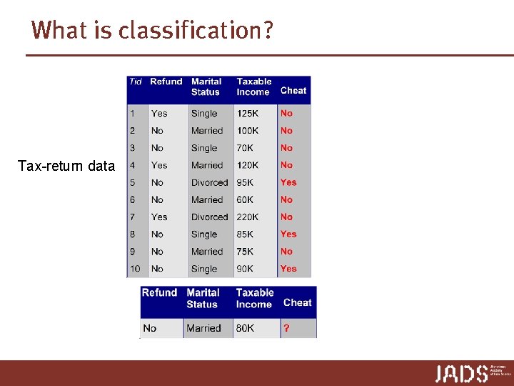
What is classification? Tax-return data

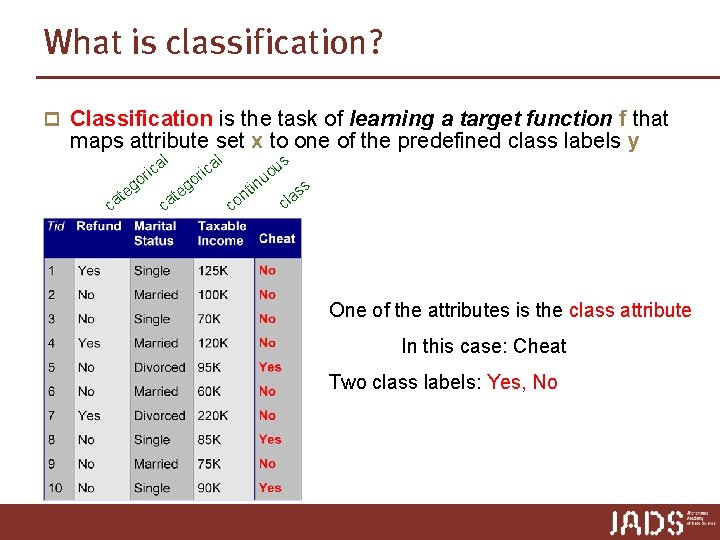
What is classification? p Classification is the task of learning a target function f that maps attribute set x to one of the predefined class labels y te ca l a c ri o g l e at c s ica r go in u uo c t on ss cla One of the attributes is the class attribute In this case: Cheat Two class labels: Yes, No

Examples of Classification Task p Predicting tumor cells as benign or malignant p Classifying credit card transactions as legitimate or fraudulent p Categorizing news stories as finance, weather, entertainment, sports, etc p Identifying spam email, spam web pages, adult content p Categorizing web users, and web queries

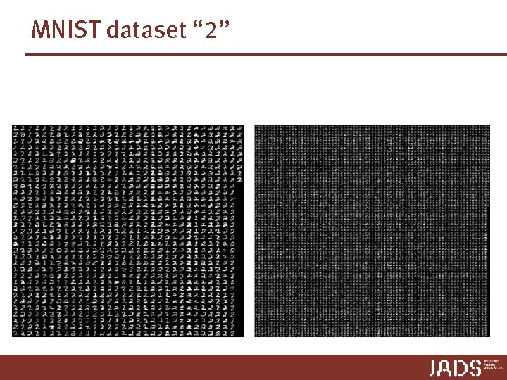
MNIST dataset “ 2”

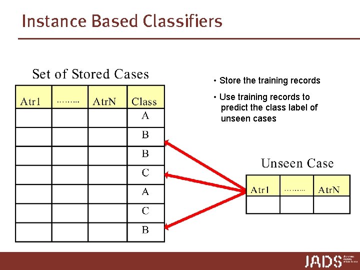
Instance Based Classifiers • Store the training records • Use training records to predict the class label of unseen cases

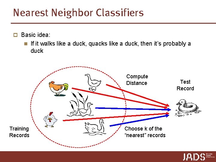
Nearest Neighbor Classifiers p Basic idea: n If it walks like a duck, quacks like a duck, then it’s probably a duck Compute Distance Training Records Choose k of the “nearest” records Test Record

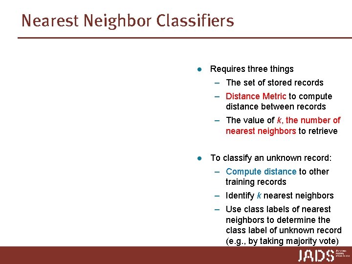
Nearest Neighbor Classifiers l Requires three things – The set of stored records – Distance Metric to compute distance between records – The value of k, the number of nearest neighbors to retrieve l To classify an unknown record: – Compute distance to other training records – Identify k nearest neighbors – Use class labels of nearest neighbors to determine the class label of unknown record (e. g. , by taking majority vote)

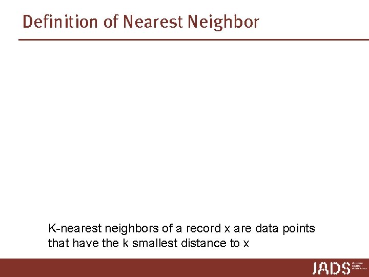
Definition of Nearest Neighbor K-nearest neighbors of a record x are data points that have the k smallest distance to x

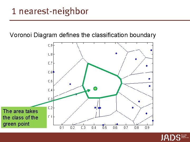
1 nearest-neighbor Voronoi Diagram defines the classification boundary The area takes the class of the green point

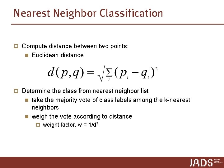
Nearest Neighbor Classification p Compute distance between two points: n Euclidean distance p Determine the class from nearest neighbor list n take the majority vote of class labels among the k-nearest neighbors n weigh the vote according to distance p weight factor, w = 1/d 2

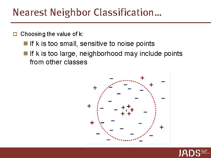
Nearest Neighbor Classification… p Choosing the value of k: n If k is too small, sensitive to noise points n If k is too large, neighborhood may include points from other classes

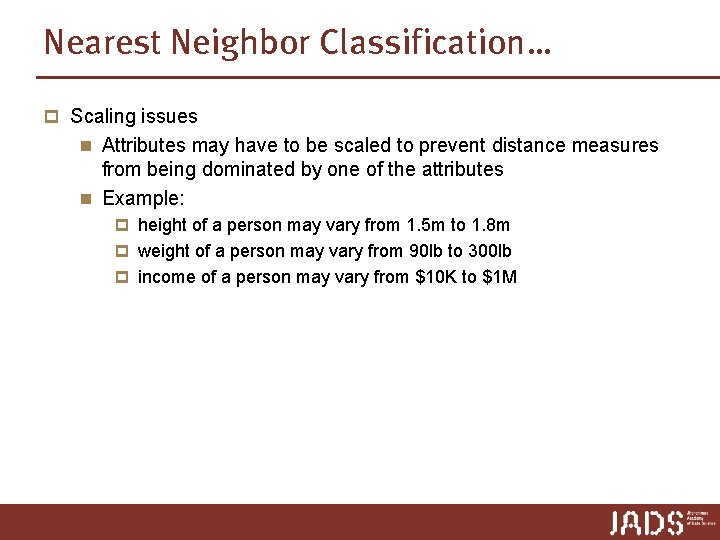
Nearest Neighbor Classification… p Scaling issues n Attributes may have to be scaled to prevent distance measures from being dominated by one of the attributes n Example: p height of a person may vary from 1. 5 m to 1. 8 m p weight of a person may vary from 90 lb to 300 lb p income of a person may vary from $10 K to $1 M

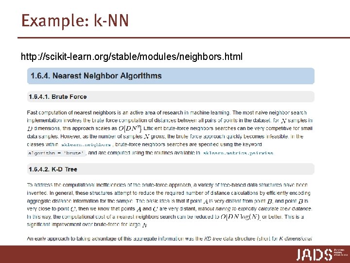
Example: k-NN http: //scikit-learn. org/stable/modules/neighbors. html

Methods for computing NN p Linear scan: O(nd) time p In practice (and medium dimension): n kd-trees work “well” in “low-medium” dimensions

Nearest neighbor Classification… p Classifying unknown records are relatively expensive n Naïve algorithm: O(n) n Need for structures to retrieve nearest neighbors fast. p The Nearest Neighbor Search problem. p Two-dimensional kd-trees n A data structure for answering nearest neighbor queries in R 2 n Answers k-nearest neighbor queries in O(k log n) time under suitable assumptions (e. g. , uniformly distributed points) n We will come back to how to perform queries later … … lets first look at a completely different problem … n How fast can we report all days with average degree between 0 - 5°, and at most 0. 5 mm of rain?

Range Searching

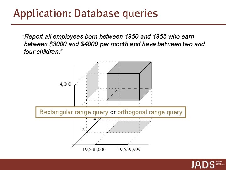
Application: Database queries Example: Database for personnel administration (name, address, date of birth, salary, …) Query: Report all employees born between 1950 and 1955 who earn between $3000 and $4000 per month. More parameters? Report all employees born between 1950 and 1955 who earn between $3000 and $4000 per month and have between two and four children. ➨ more dimensions

Application: Database queries “Report all employees born between 1950 and 1955 who earn between $3000 and $4000 per month and have between two and four children. ” Rectangular range query or orthogonal range query

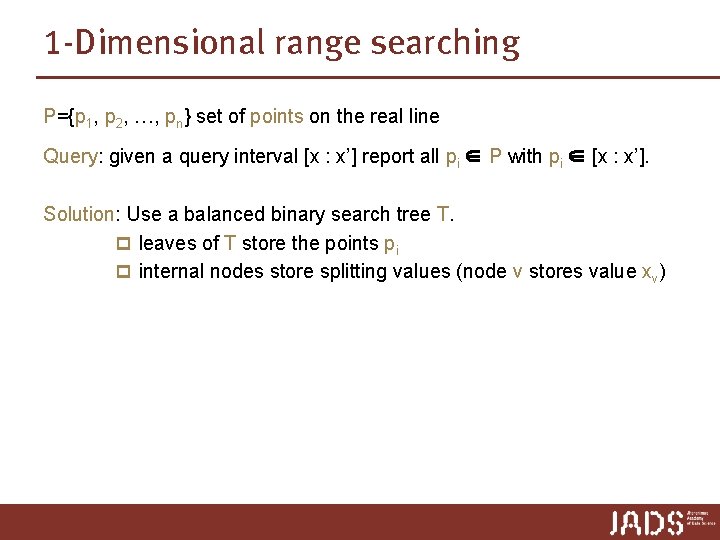
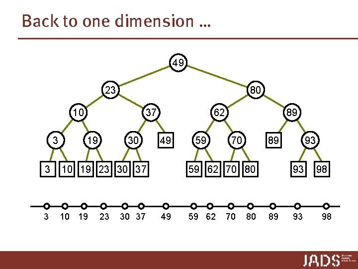
1 -Dimensional range searching P={p 1, p 2, …, pn} set of points on the real line Query: given a query interval [x : x’] report all pi ∈ P with pi ∈ [x : x’]. Solution: Use a balanced binary search tree T. p leaves of T store the points pi p internal nodes store splitting values (node v stores value xv)

1 -Dimensional range searching Query [x : x’] ➨ search with x and x’ ➨ end in two leaves μ and μ’ Report 1. all leaves between μ and μ’ 2. possibly points stored at μ and μ’ [18 : 77] 49 23 80 10 3 3 37 19 30 10 19 23 30 37 μ 62 49 59 89 70 93 89 59 62 70 80 μ’ 93 98

1 -Dimensional range searching Query [x : x’] ➨ search with x and x’ ➨ end in two leaves μ and μ’ Report 1. all leaves between μ and μ’ 2. possibly points stored at μ and μ’ [18 : 77] 49 23 80 How do we find all leaves between μ and μ’? 10 37 62 89 3 3 19 30 10 19 23 30 37 μ 49 59 70 93 89 59 62 70 80 μ’ 93 98

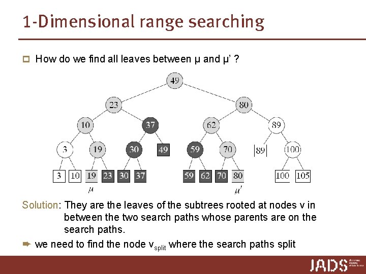
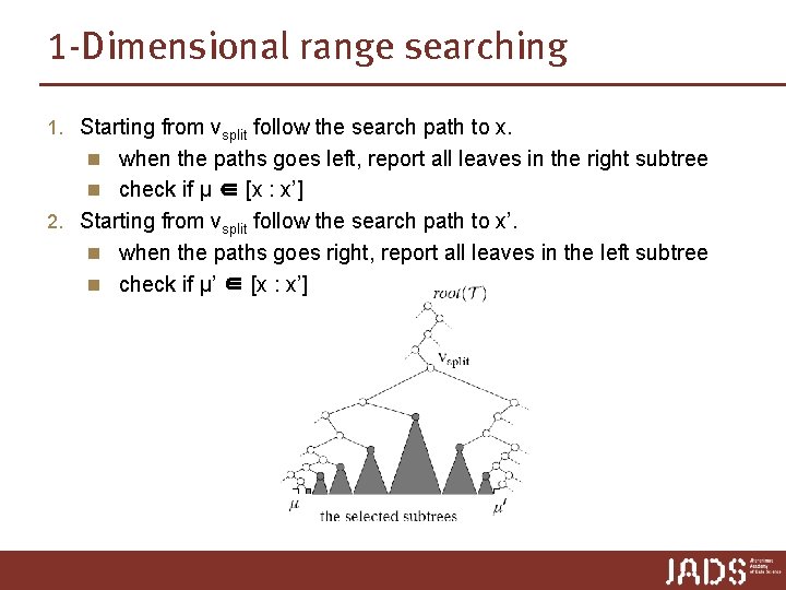
1 -Dimensional range searching p How do we find all leaves between μ and μ’ ? Solution: They are the leaves of the subtrees rooted at nodes v in between the two search paths whose parents are on the search paths. ➨ we need to find the node vsplit where the search paths split

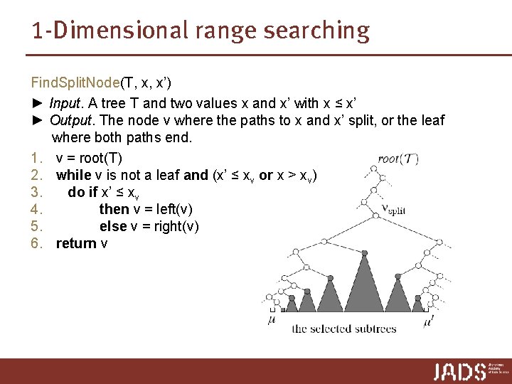
1 -Dimensional range searching Find. Split. Node(T, x, x’) ► Input. A tree T and two values x and x’ with x ≤ x’ ► Output. The node v where the paths to x and x’ split, or the leaf where both paths end. 1. v = root(T) 2. while v is not a leaf and (x’ ≤ xv or x > xv) 3. do if x’ ≤ xv 4. then v = left(v) 5. else v = right(v) 6. return v

1 -Dimensional range searching 1. Starting from vsplit follow the search path to x. n when the paths goes left, report all leaves in the right subtree n check if µ ∈ [x : x’] 2. Starting from vsplit follow the search path to x’. n when the paths goes right, report all leaves in the left subtree n check if µ’ ∈ [x : x’]

1 -Dimensional range searching 1 DRange. Query(T, [x : x’]) ► Input. A binary search tree T and a range [x : x’]. ► Output. All points stored in T that lie in the range. 1. vsplit = Find. Split. Node(T, x, x’) 2. if vsplit is a leaf 3. then Check if the point stored at vsplit must be reported. 4. else (Follow the path to x and report the points in subtrees right of the path) 5. v = left(vsplit) 6. while v is not a leaf 7. do if x ≤ xv 8. then Report. Subtree(right(v)) 9. v = left(v) 10. else v = right(v) 11. Check if the point stored at the leaf v must be reported. 12. Similarly, follow the path to x’, report the points in subtrees left of the path, and check if the point stored at the leaf where the path ends must be reported.

1 -Dimensional range searching 1 DRange. Query(T, [x, x’]) ► Input. A binary search tree T and a range [x : x’]. ► Output. All points stored in T that lie in the range. 1. vsplit = Find. Split. Node(T, x, x’) 2. if vsplit is a leaf 3. then Check if the point stored at vsplit must be reported. 4. else (Follow the path to x and report the points in subtrees right of the path) 5. v = left(vsplit) 6. while v is not a leaf 7. do if x ≤ xv 8. then Report. Subtree(right(v)) 9. v = left(v) 10. else v = right(v) 11. Check if the point stored at the leaf v must be reported. 12. Similarly, follow the path to x’, report the points in subtrees left of the path, and check if the point stored at the leaf where the path ends must be reported. Correctness? Need to show two things: 1. every reported point lies in the query range 2. every point in the query range is reported.

1 -Dimensional range searching 1 DRange. Query(T, [x, x’]) ► Input. A binary search tree T and a range [x : x’]. ► Output. All points stored in T that lie in the range. 1. vsplit = Find. Split. Node(T, x, x’) 2. if vsplit is a leaf 3. then Check if the point stored at vsplit must be reported. 4. else (Follow the path to x and report the points in subtrees right of the path) 5. v = left(vsplit) 6. while v is not a leaf 7. do if x ≤ xv 8. then Report. Subtree(right(v)) 9. v = left(v) 10. else v = right(v) 11. Check if the point stored at the leaf v must be reported. 12. Similarly, follow the path to x’, report the points in subtrees left of the path, and check if the point stored at the leaf where the path ends must be reported. Query time? Report. Subtree = O(1 + reported points) ➨ total query time = O(log n + reported points) Storage? O(n)

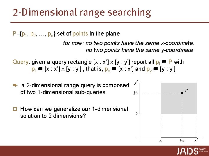
2 -Dimensional range searching P={p 1, p 2, …, pn} set of points in the plane for now: no two points have the same x-coordinate, no two points have the same y-coordinate Query: given a query rectangle [x : x’] x [y : y’] report all pi ∈ P with pi ∈ [x : x’] x [y : y’] , that is, px ∈ [x : x’] and py ∈ [y : y’] ➨ a 2 -dimensional range query is composed of two 1 -dimensional sub-queries p How can we generalize our 1 -dimensional solution to 2 dimensions?

Back to one dimension … 49 23 80 10 3 37 19 30 3 10 19 23 30 37 62 49 59 89 70 59 62 70 80 49 59 62 70 93 89 80 93 89 93 98 98

Back to one dimension … 49 23 80 10 3 37 19 30 3 10 19 23 30 37 62 49 59 89 70 59 62 70 80 49 59 62 70 93 89 80 93 89 93 98 98

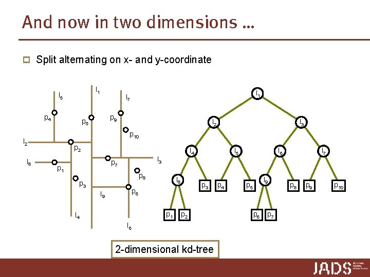
And now in two dimensions … p Split alternating on x- and y-coordinate l 1 l 5 p 4 p 9 p 5 l 2 l 3 p 10 l 2 l 8 l 1 l 7 p 2 l 3 p 7 p 1 l 4 p 8 p 3 l 8 p 3 p 6 l 9 p 1 l 4 l 5 p 2 l 6 2 -dimensional kd-tree p 4 l 6 l 9 p 5 p 6 p 7 l 7 p 8 p 9 p 10

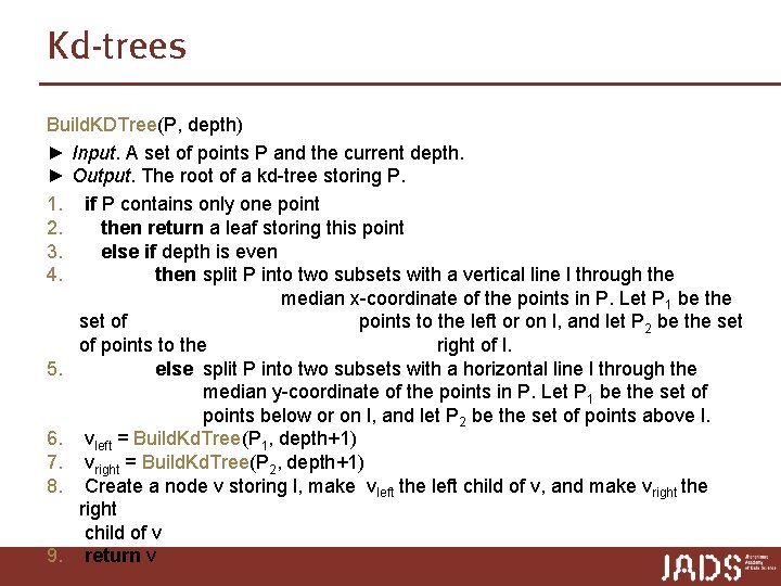
Kd-trees Build. KDTree(P, depth) ► Input. A set of points P and the current depth. ► Output. The root of a kd-tree storing P. 1. if P contains only one point 2. then return a leaf storing this point 3. else if depth is even 4. then split P into two subsets with a vertical line l through the median x-coordinate of the points in P. Let P 1 be the set of points to the left or on l, and let P 2 be the set of points to the right of l. 5. else split P into two subsets with a horizontal line l through the median y-coordinate of the points in P. Let P 1 be the set of points below or on l, and let P 2 be the set of points above l. 6. vleft = Build. Kd. Tree(P 1, depth+1) 7. vright = Build. Kd. Tree(P 2, depth+1) 8. Create a node v storing l, make vleft the left child of v, and make vright the right child of v 9. return v

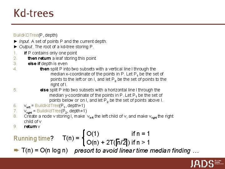
Kd-trees Build. KDTree(P, depth) ► Input. A set of points P and the current depth. ► Output. The root of a kd-tree storing P. 1. if P contains only one point 2. then return a leaf storing this point 3. else if depth is even 4. then split P into two subsets with a vertical line l through the median x-coordinate of the points in P. Let P 1 be the set of points to the left or on l, and let P 2 be the set of points to the right of l. 5. else split P into two subsets with a horizontal line l through the median y-coordinate of the points in P. Let P 1 be the set of points below or on l, and let P 2 be the set of points above l. 6. vleft = Build. Kd. Tree(P 1, depth+1) 7. vright = Build. Kd. Tree(P 2, depth+1) 8. Create a node v storing l, make vleft the left child of v, and make vright the right child of v 9. return v Running time? O(1) if n = 1 O(n) + 2 T( n/2 ) if n > 1 presort to avoid linear time median finding … T(n) = ➨ T(n) = O(n log n)

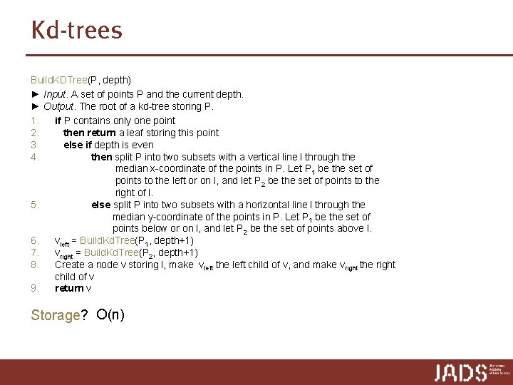
Kd-trees Build. KDTree(P, depth) ► Input. A set of points P and the current depth. ► Output. The root of a kd-tree storing P. 1. if P contains only one point 2. then return a leaf storing this point 3. else if depth is even 4. then split P into two subsets with a vertical line l through the median x-coordinate of the points in P. Let P 1 be the set of points to the left or on l, and let P 2 be the set of points to the right of l. 5. else split P into two subsets with a horizontal line l through the median y-coordinate of the points in P. Let P 1 be the set of points below or on l, and let P 2 be the set of points above l. 6. vleft = Build. Kd. Tree(P 1, depth+1) 7. vright = Build. Kd. Tree(P 2, depth+1) 8. Create a node v storing l, make vleft the left child of v, and make vright the right child of v 9. return v Storage? O(n)

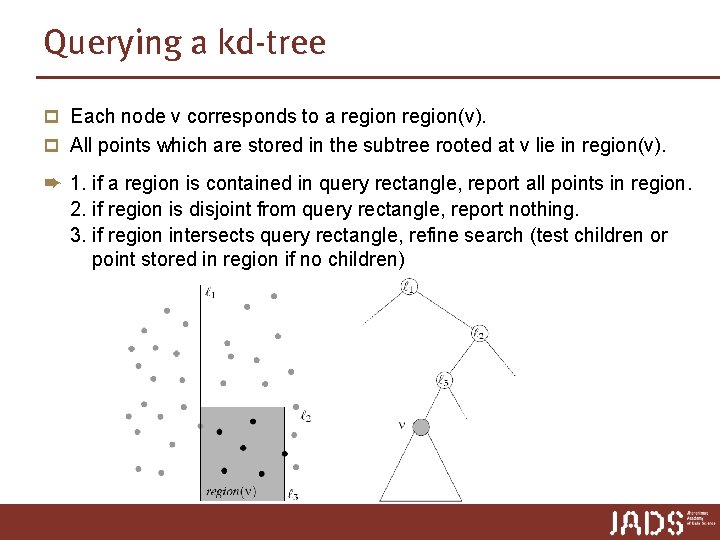
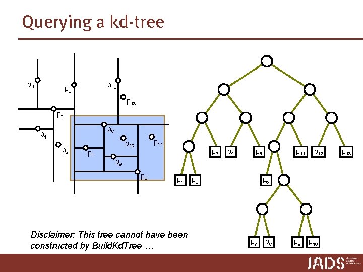
Querying a kd-tree p Each node v corresponds to a region(v). p All points which are stored in the subtree rooted at v lie in region(v). ➨ 1. if a region is contained in query rectangle, report all points in region. 2. if region is disjoint from query rectangle, report nothing. 3. if region intersects query rectangle, refine search (test children or point stored in region if no children)

Querying a kd-tree p 4 p 12 p 5 p 13 p 2 p 8 p 1 p 3 p 11 p 10 p 7 p 3 p 4 p 5 p 11 p 12 p 9 p 6 p 1 Disclaimer: This tree cannot have been constructed by Build. Kd. Tree … p 2 p 6 p 7 p 8 p 9 p 10 p 13

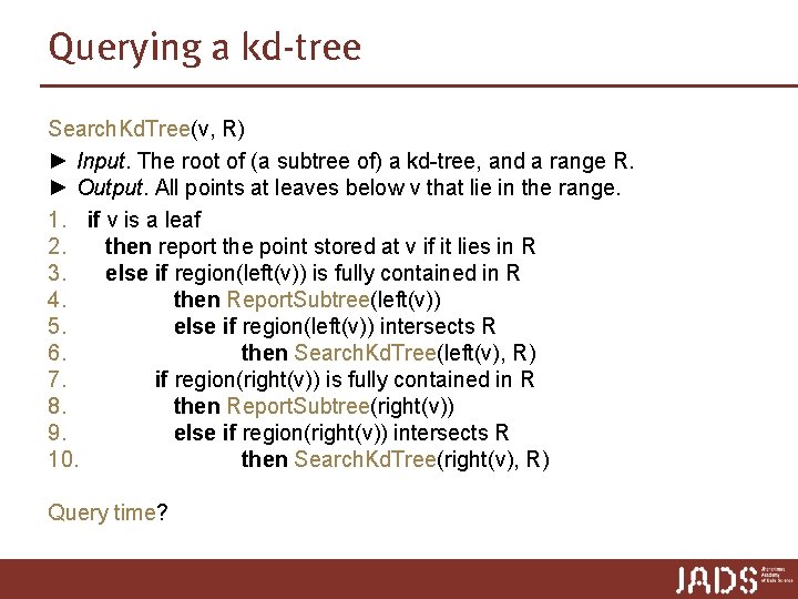
Querying a kd-tree Search. Kd. Tree(v, R) ► Input. The root of (a subtree of) a kd-tree, and a range R. ► Output. All points at leaves below v that lie in the range. 1. if v is a leaf 2. then report the point stored at v if it lies in R 3. else if region(left(v)) is fully contained in R 4. then Report. Subtree(left(v)) 5. else if region(left(v)) intersects R 6. then Search. Kd. Tree(left(v), R) 7. if region(right(v)) is fully contained in R 8. then Report. Subtree(right(v)) 9. else if region(right(v)) intersects R 10. then Search. Kd. Tree(right(v), R) Query time?

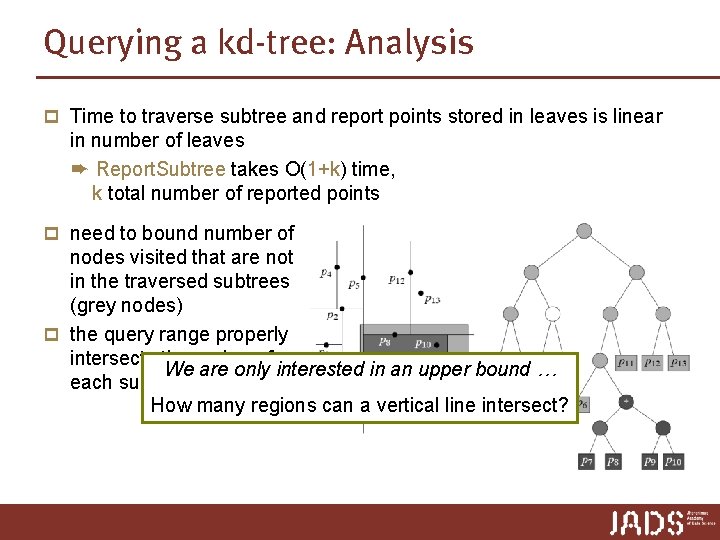
Querying a kd-tree: Analysis p Time to traverse subtree and report points stored in leaves is linear in number of leaves ➨ Report. Subtree takes O(1+k) time, k total number of reported points p need to bound number of nodes visited that are not in the traversed subtrees (grey nodes) p the query range properly intersects the region of We are only interested in an upper bound … each such node How many regions can a vertical line intersect?

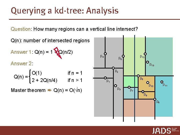
Querying a kd-tree: Analysis Question: How many regions can a vertical line intersect? Q(n): number of intersected regions Answer 1: Q(n) = 1 + Q(n/2) p 4 p 12 p 5 Answer 2: O(1) Q(n) = 2 + 2 Q(n/4) p 13 if n = 1 if n > 1 Master theorem ➨ Q(n) = O(√n) p 2 p 8 p 1 p 3 p 11 p 10 p 7 p 9 p 6

KD-trees Theorem A kd-tree for a set of n points in the plane uses O(n) storage and can be built in O(n log n) time. A rectangular range query on the kdtree takes O(√n + k) time, where k is the number of reported points. Generalizes to dimension d: O(n 1 -1/d + k), but high dependency on dimension.

Back to: Nearest Neighbor Searching

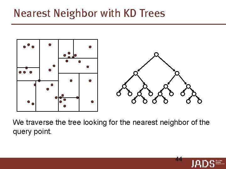
Nearest Neighbor with KD Trees We traverse the tree looking for the nearest neighbor of the query point. 44

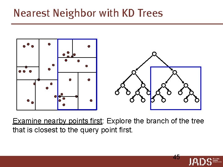
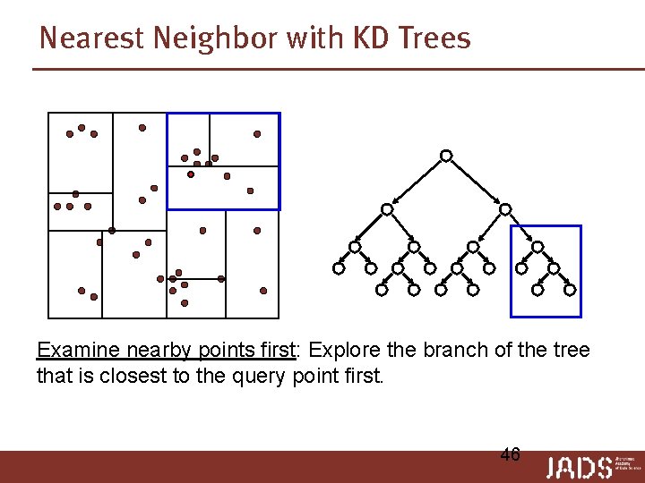
Nearest Neighbor with KD Trees Examine nearby points first: Explore the branch of the tree that is closest to the query point first. 45

Nearest Neighbor with KD Trees Examine nearby points first: Explore the branch of the tree that is closest to the query point first. 46

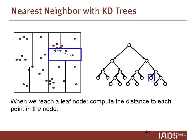
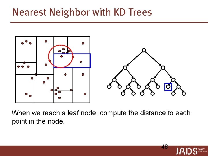
Nearest Neighbor with KD Trees When we reach a leaf node: compute the distance to each point in the node. 47

Nearest Neighbor with KD Trees When we reach a leaf node: compute the distance to each point in the node. 48

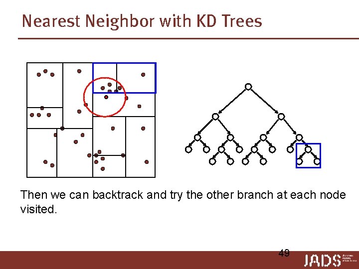
Nearest Neighbor with KD Trees Then we can backtrack and try the other branch at each node visited. 49

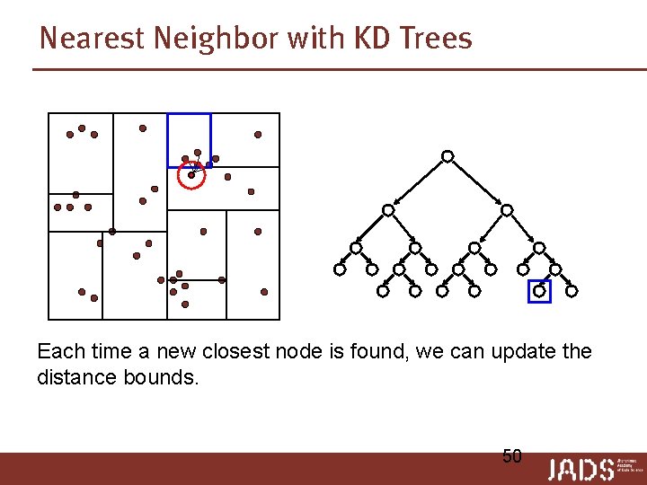
Nearest Neighbor with KD Trees Each time a new closest node is found, we can update the distance bounds. 50

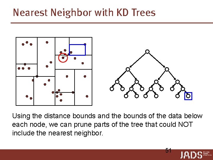
Nearest Neighbor with KD Trees Using the distance bounds and the bounds of the data below each node, we can prune parts of the tree that could NOT include the nearest neighbor. 51

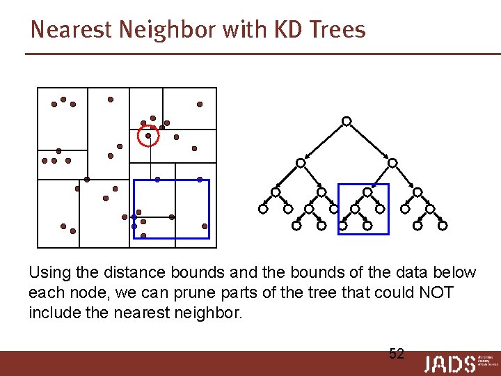
Nearest Neighbor with KD Trees Using the distance bounds and the bounds of the data below each node, we can prune parts of the tree that could NOT include the nearest neighbor. 52

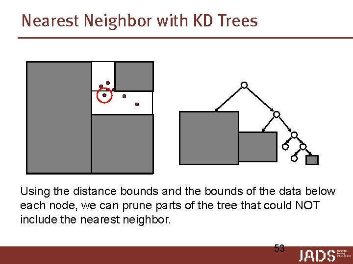
Nearest Neighbor with KD Trees Using the distance bounds and the bounds of the data below each node, we can prune parts of the tree that could NOT include the nearest neighbor. 53

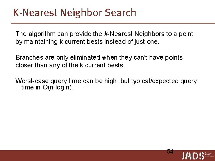
K-Nearest Neighbor Search The algorithm can provide the k-Nearest Neighbors to a point by maintaining k current bests instead of just one. Branches are only eliminated when they can't have points closer than any of the k current bests. Worst-case query time can be high, but typical/expected query time in O(n log n). 54

Recap and preview Today p Kd-trees n Range searching n Nearest Neighbor searching Next lectures p Practice Exam