Data Structures Algorithms Lecture 12 b WrapUp The

Data Structures & Algorithms Lecture 12 b: Wrap-Up

The course p Design and analysis of efficient algorithms for some basic computational problems. n Basic algorithm design techniques and paradigms n Algorithms analysis: O-notation, recursions, … n Basic data structures n Basic searching and sorting algorithms n Basic graph algorithms

Algorithm Paradigms Incremental algorithms process the input elements one-by-one and maintain the solution for the elements processed so far. Divide-and-conquer break the problem into two or more subproblems, solve the subproblems recursively, and then combine these solutions to create a solution to the original problem. In practice: often a combination of both.

Describing algorithms p A complete description of an algorithm consists of three parts: 1. the algorithm (expressed in whatever way is clearest and most concise, can be English and / or pseudocode) 2. a proof of the algorithm’s correctness 3. a derivation of the algorithm’s running time

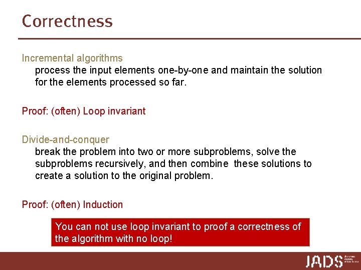
Correctness Incremental algorithms process the input elements one-by-one and maintain the solution for the elements processed so far. Proof: (often) Loop invariant Divide-and-conquer break the problem into two or more subproblems, solve the subproblems recursively, and then combine these solutions to create a solution to the original problem. Proof: (often) Induction You can not use loop invariant to proof a correctness of the algorithm with no loop!

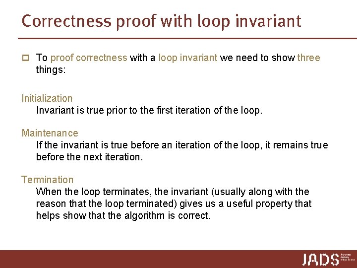
Correctness proof with loop invariant p To proof correctness with a loop invariant we need to show three things: Initialization Invariant is true prior to the first iteration of the loop. Maintenance If the invariant is true before an iteration of the loop, it remains true before the next iteration. Termination When the loop terminates, the invariant (usually along with the reason that the loop terminated) gives us a useful property that helps show that the algorithm is correct.

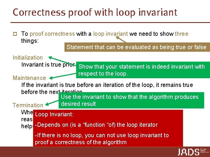
Correctness proof with loop invariant p To proof correctness with a loop invariant we need to show three things: Statement that can be evaluated as being true or false Initialization Invariant is true prior to. Show the first of the loop. thatiteration your statement is indeed invariant with respect to the loop. Maintenance If the invariant is true before an iteration of the loop, it remains true before the next iteration. Use the invariant to show that the algorithm produces desired result Termination When. Loop the loop terminates, the invariant (usually along with the Invariant: reason that the loop terminated) gives us a useful property that Depends a “function “of) the loop iterator helps-show thaton the(is algorithm is correct. -If there is no loop, you can not use loop invariant to proof a correctness of the algorithm

Example: insertion sort Insertion. Sort(A) 1. initialize: sort A[1] 2. for j ← 2 to length[A] 3. do key ← A[j] 4. i ← j -1 5. while i > 0 and A[i] > key 6. do A[i+1] ← A[i] 7. i ← i -1 8. A[i +1] ← key Loop invariant At the start of each iteration of the “outer” for loop (indexed by j) the subarray A[1. . j-1] consists of the elements originally in A[1. . j-1] but in sorted order.

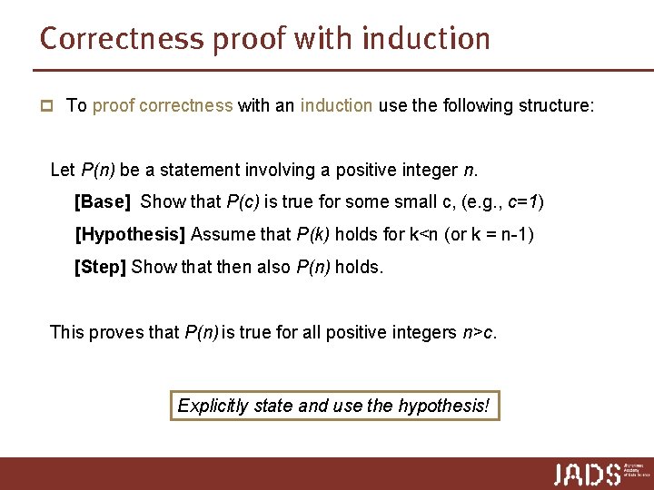
Correctness proof with induction p To proof correctness with an induction use the following structure: Let P(n) be a statement involving a positive integer n. [Base] Show that P(c) is true for some small c, (e. g. , c=1) [Hypothesis] Assume that P(k) holds for k<n (or k = n-1) [Step] Show that then also P(n) holds. This proves that P(n) is true for all positive integers n>c. Explicitly state and use the hypothesis!

Merge. Sort: correctness proof Merge. Sort(A) 1. if length[A] = 1 2. then skip 3. else 4. n = A. length ; n 1 = n/2 ; n 2 = n/2 ; copy A[1. . n 1] to auxiliary array A 1[1. . n 1] copy A[n 1+1. . n] to auxiliary array A 2[1. . n 2] 5. Merge. Sort(A 1) Lemma 6. Merge. Sort(A 2) Merge. Sort 7. Merge(A, A 1, A 2) sorts the array A[1. . n] correctly. Proof (by induction on n) Base case: n = 1, trivial ✔ Inductive step: assume n > 1. Note that n 1 < n and n 2 < n. Inductive hypothesis ➨ arrays A 1 and A 2 are sorted correctly Remains to show: Merge(A, A 1, A 2) correctly constructs a sorted array A out of the sorted arrays A 1 and A 2 … etc. ■

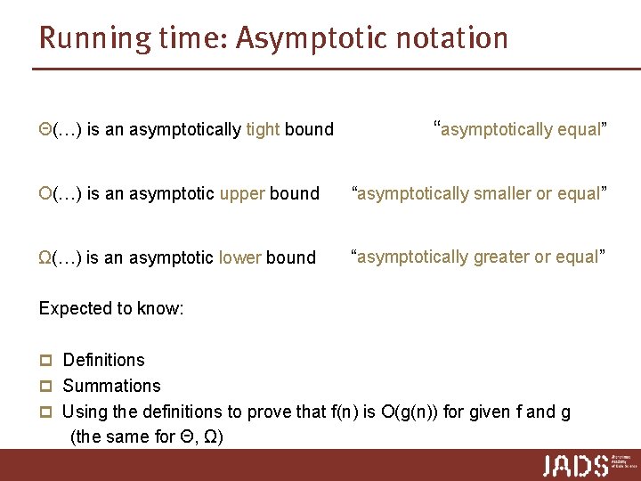
Running time: Asymptotic notation Θ(…) is an asymptotically tight bound “asymptotically equal” O(…) is an asymptotic upper bound “asymptotically smaller or equal” Ω(…) is an asymptotic lower bound “asymptotically greater or equal” Expected to know: p Definitions p Summations p Using the definitions to prove that f(n) is O(g(n)) for given f and g (the same for Θ, Ω)

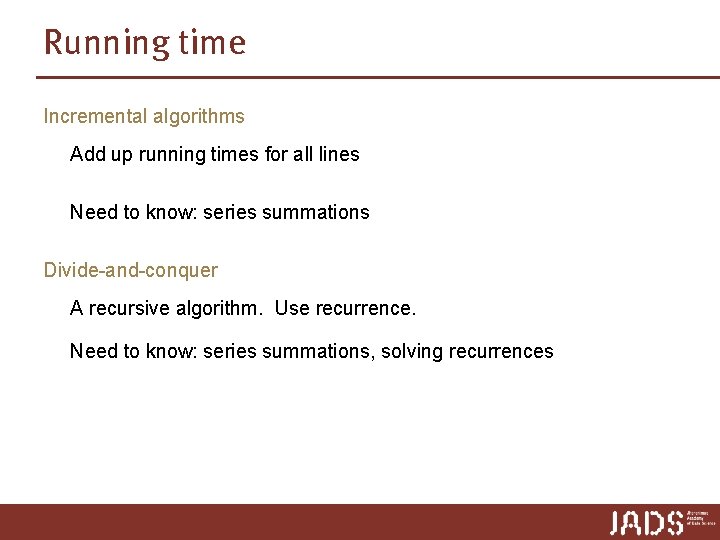
Running time Incremental algorithms Add up running times for all lines Need to know: series summations Divide-and-conquer A recursive algorithm. Use recurrence. Need to know: series summations, solving recurrences

Analysis of Insertion. Sort(A) 1. initialize: sort A[1] 2. for j ← 2 to length[A] 3. do key ← A[j] 4. i ← j -1 5. while i > 0 and A[i] > key 6. do A[i+1] ← A[i] 7. i ← i -1 8. A[i +1] ← key O(1) worst case: (j-1) ∙ O(1) Upper bound: Let T(n) be the worst case running time of Insertion. Sort on an array of length n. We have T(n) = O(1) + { O(1) + (j-1)∙O(1) + O(1) } = O(j) = O(n 2) Lower bound: Array sorted in de-creasing order ➨ Ω(n 2) The worst case running time of Insertion. Sort is Θ(n 2).

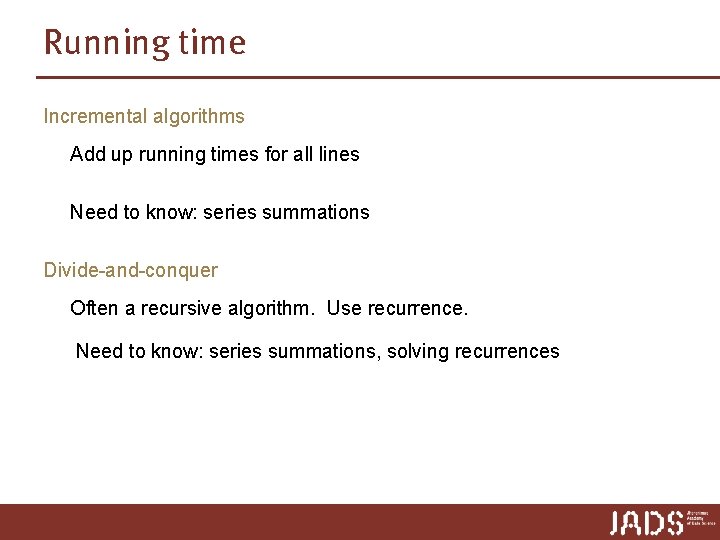
Running time Incremental algorithms Add up running times for all lines Need to know: series summations Divide-and-conquer Often a recursive algorithm. Use recurrence. Need to know: series summations, solving recurrences

Analysis of Merge. Sort(A) ► divide-and-conquer algorithm that sorts array A[1. . n] 1. if length[A] = 1 2. then skip 3. else 4. n ← length[A] ; n 1 ← floor(n/2); n 2 ← ceil(n/2); 5. copy A[1. . n 1] to auxiliary array A 1[1. . n 1] 6. copy A[n 1+1. . n] to auxiliary array A 2[1. . n 2] 7. Merge. Sort(A 1); Merge. Sort(A 2) 8. Merge(A, A 1, A 2) T( n/2 ) + T( n/2 ) Merge. Sort is a recursive algorithm ➨ running time analysis leads to recursion O(1) O(n) ? ? O(n)

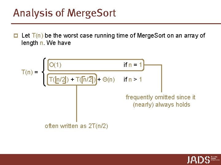
Analysis of Merge. Sort p Let T(n) be the worst case running time of Merge. Sort on an array of length n. We have O(1) if n = 1 T( n/2 ) + Θ(n) if n > 1 T(n) = frequently omitted since it (nearly) always holds often written as 2 T(n/2)

Solving recurrences p Easiest: Master theorem (the way it is given in the slides, and not other sources you might have found) caveat: not always applicable p Alternatively: draw and analyze the recursion tree p Note: No substitution method in exam

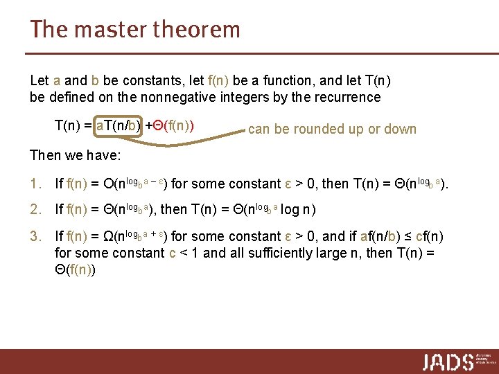
The master theorem Let a and b be constants, let f(n) be a function, and let T(n) be defined on the nonnegative integers by the recurrence T(n) = a. T(n/b) +Θ(f(n)) can be rounded up or down Then we have: 1. If f(n) = O(nlogb a – ε) for some constant ε > 0, then T(n) = Θ(nlogb a). 2. If f(n) = Θ(nlogba), then T(n) = Θ(nlogb a log n) 3. If f(n) = Ω(nlogba + ε) for some constant ε > 0, and if af(n/b) ≤ cf(n) for some constant c < 1 and all sufficiently large n, then T(n) = Θ(f(n))

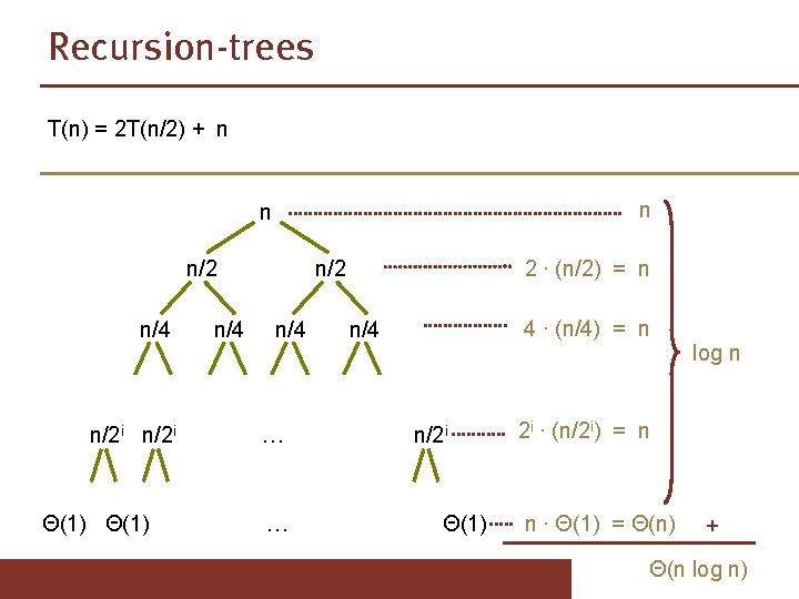
Recursion-trees T(n) = 2 T(n/2) + n n/2 n/4 n/2 i Θ(1) n/4 n/2 n/4 … … 2 ∙ (n/2) = n 4 ∙ (n/4) = n n/4 n/2 i Θ(1) log n 2 i ∙ (n/2 i) = n n ∙ Θ(1) = Θ(n) + Θ(n log n)

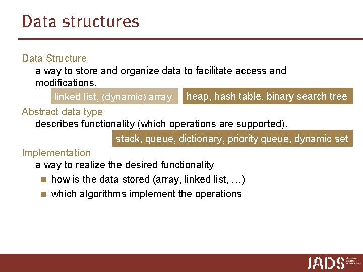
Data structures Data Structure a way to store and organize data to facilitate access and modifications. linked list, (dynamic) array heap, hash table, binary search tree Abstract data type describes functionality (which operations are supported). stack, queue, dictionary, priority queue, dynamic set Implementation a way to realize the desired functionality n how is the data stored (array, linked list, …) n which algorithms implement the operations

Data structures Abstract data types: p Which data structures support of a given abstract data how efficient the required operations are n E. g. dictionary can be implemented as BST, hash table, sorted array n Which data structure realizes it in the most efficient way etc. Data structures: p Which Data Structures efficiently supports which operations n E. g. heap supports priority queue operations n Binary Search tree supports both priority queue and dictionary n Hash table supports dictionary

Data structures: p Properties of each data structure n Running time for basic operations n The way operations are implemented n Other (e. g. BST property, heap property etc) In general: properties of the structure that enable us to implement required operations efficiently

Sorting algorithms Insertion. Sort, Merge. Sort, Heap. Sort, Counting. Sort, Radix. Sort, Quicksort p How each of them works p Requirements towards the input n Integer input n Within a certain range p Basic properties n in place n Stable n Running time n Paradigm: Incremental/divide-and-conquer

Implementing Dictionary and Dynamic Set p Hash tables implement Dictionary n Open adressing vs. chaining n Running times of operations p Binary Search trees implement Dynamic Set n Binary search tree property n Running times of operations

Graph Algorithms p Graphs n Definitions and concepts n Graph representations p BFS, DFS n How they work n Running times p Topological sort n definition n when does it exists n Algorithm p Single-Source Shortest Path: Dijkstra

Advanced topics p p What you don’t need to know in the exam … Substitution method How to balance a binary search tree n Weight-balanced: BB[α]-trees n Height-balanced: AVL-trees, red-black trees n Degree-balanced: (2, 3)-tree n … but you should know: we can maintain a balanced BSTs and then height = O(log n) Complexity classes for algorithmic problems n Traveling salesperson problem n NP-completeness Range trees n Range queries n Nearest Neighbor queries

Tips p Chose the right data structure for your problem p Think of which operations you need to access/update your data p Why one data structure fits your purpose better than the other etc p Try to think whether you can use (directly or indirectly) an existing algorithm for solving your problem

Exam p Expect n all algorithmic topics/data structures to occur (more or less n n n prominently), except possibly shortest path algorithms asymptotic analysis, correctness not too many inductions comparison of data structures executing algorithms 8 -10 questions: 1 -2 easy, 1 -2 hard (e. g. , algorithm design)