Data Structures Algorithms Lecture 1 Linear Search Proofs

Data Structures & Algorithms Lecture 1: Linear Search & Proofs

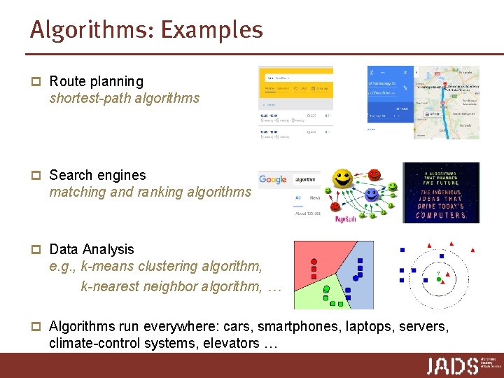
Algorithms: Examples p Route planning shortest-path algorithms p Search engines matching and ranking algorithms p Data Analysis e. g. , k-means clustering algorithm, k-nearest neighbor algorithm, … p Algorithms run everywhere: cars, smartphones, laptops, servers, climate-control systems, elevators …

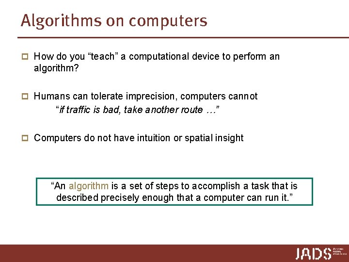
Algorithms on computers p How do you “teach” a computational device to perform an algorithm? p Humans can tolerate imprecision, computers cannot “if traffic is bad, take another route …” p Computers do not have intuition or spatial insight “An algorithm is a set of steps to accomplish a task that is described precisely enough that a computer can run it. ”

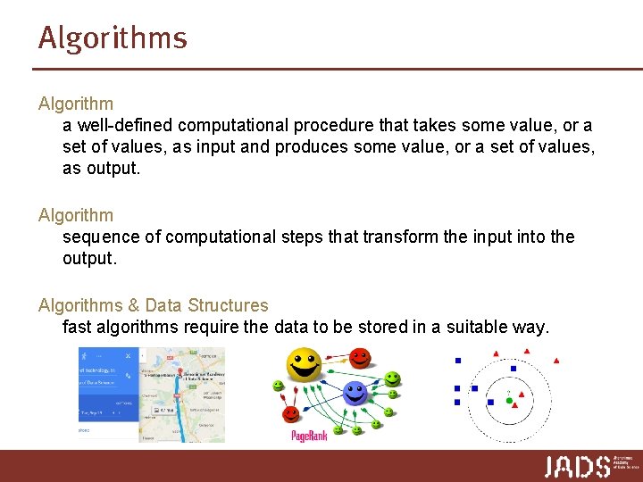
Algorithms Algorithm a well-defined computational procedure that takes some value, or a set of values, as input and produces some value, or a set of values, as output. Algorithm sequence of computational steps that transform the input into the output. Algorithms & Data Structures fast algorithms require the data to be stored in a suitable way.

Data structures Data Structure a way to store and organize data to facilitate access and modifications. Abstract data type describes functionality (which operations are supported). Implementation a way to realize the desired functionality n how is the data stored (array, linked list, …) n which algorithms implement the operations

The course: Overview p Design and analysis of efficient algorithms for some basic computational problems. n Basic algorithm design techniques and paradigms n Algorithms analysis: O-notation, recursions, … n Basic data structures n Basic graph algorithms

The course: Objectives For any computational task on data you need an algorithm to solve it, and you need to store the data in a suitable data structure to access the data. If the data are large, you need these algorithms and data structures to be efficient. At the end of this course, you should be able: p select a suitable basic algorithm and data structure for a given task p design efficient algorithms for simple computational tasks

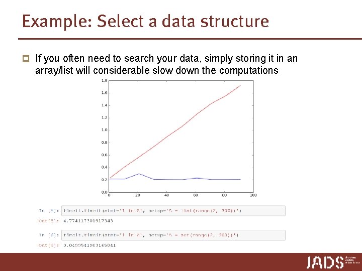
Example: Select a data structure p If you often need to search your data, simply storing it in an array/list will considerable slow down the computations

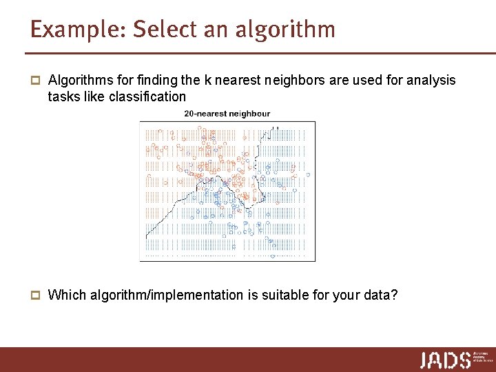
Example: Select an algorithm p Algorithms for finding the k nearest neighbors are used for analysis tasks like classification p Which algorithm/implementation is suitable for your data?

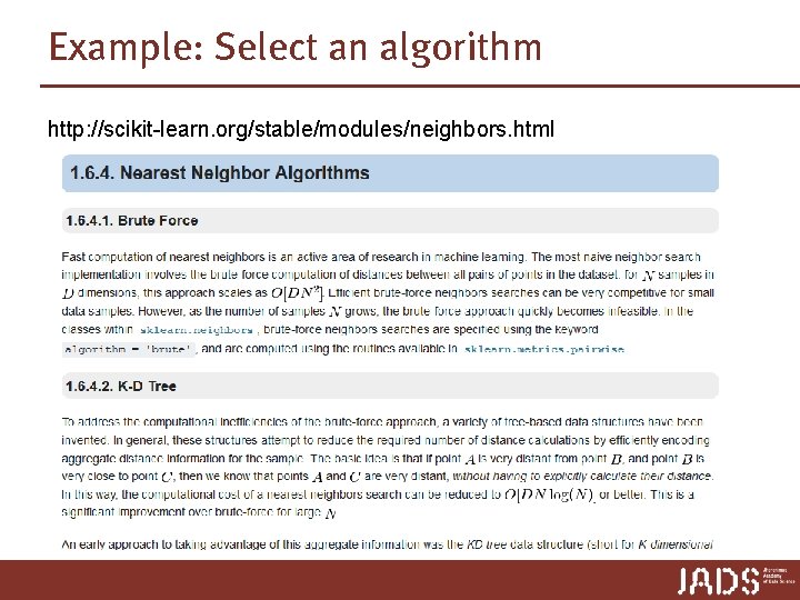
Example: Select an algorithm http: //scikit-learn. org/stable/modules/neighbors. html

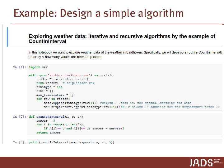
Example: Design a simple algorithm

Some administration first before we really get started …

Organization Instructor: Dr. Kevin Buchin, TU Eindhoven, k. a. buchin@tue. nl, use tag [JBP 030] in e-mails Web page: http: //www. win. tue. nl/~kbuchin/teaching/JBP 031/ slides, assignment, … will be posted on the webpage

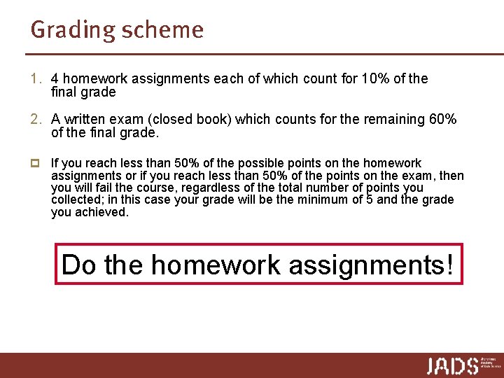
Grading scheme 1. 4 homework assignments each of which count for 10% of the final grade 2. A written exam (closed book) which counts for the remaining 60% of the final grade. p If you reach less than 50% of the possible points on the homework assignments or if you reach less than 50% of the points on the exam, then you will fail the course, regardless of the total number of points you collected; in this case your grade will be the minimum of 5 and the grade you achieved. Do the homework assignments!

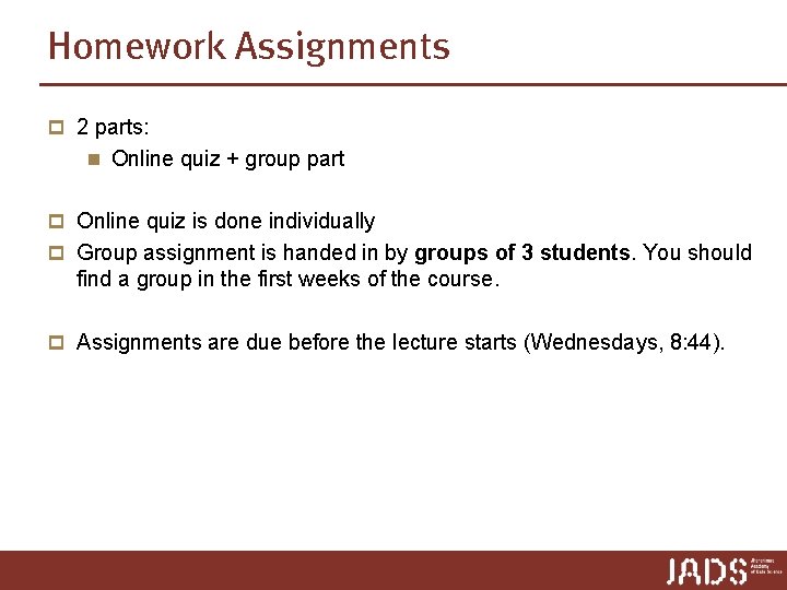
Homework Assignments p 2 parts: n Online quiz + group part p Online quiz is done individually p Group assignment is handed in by groups of 3 students. You should find a group in the first weeks of the course. p Assignments are due before the lecture starts (Wednesdays, 8: 44).

Group Part of Assignment p Homework assignments have to be written in English. n You can hand in your solution electronically as a pdf n I recommend writing your solution as Jupyter Notebook (as soon as you learned about them), since this makes it easy to type mathematical expressions and include python code. p Use blackboard to hand in your solution. In case of a Jupyter Notebook hand in the Jupyter Notebook as such and saved as pdf p Note: solutions “inspired” by existing solutions to a problem are not considered. If you present ideas or even (partial) solutions as your own, it is considered fraud, and handled accordingly. If you are stuck on a problem, feel free to ask me about it.

Online Quiz p Uses oncourse. tue. nl p First you will need your TU/e account, therefore quiz is not posted yet p Then you need to self-enroll to the corresponding course: https: //oncourse. tue. nl/2018/course/view. php? id=76, for this you need the enrollment key (posted on blackboard) p You can test the environment using Quiz 0 is not an assignment, and does not contribute to final grade p This is a pilot. Please report issues, feedback is welcome!

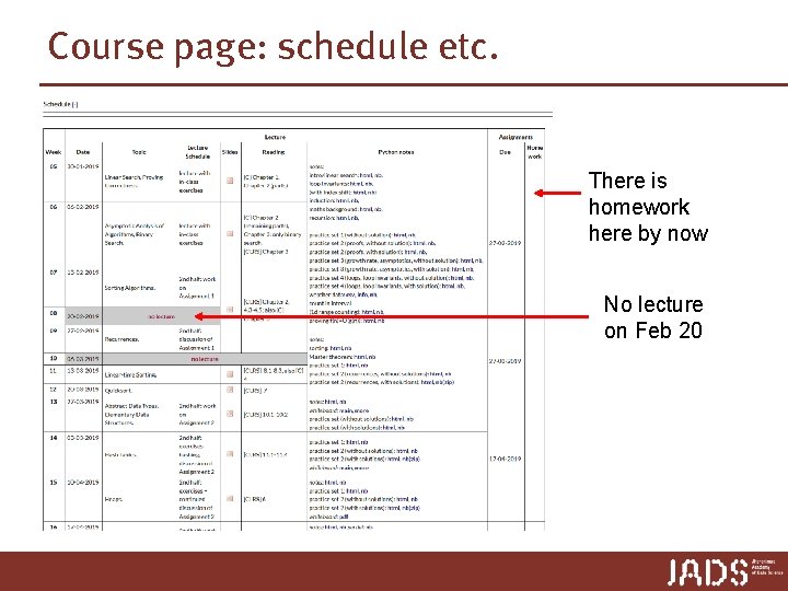
Course page: schedule etc. There is homework here by now No lecture on Feb 20

Books p You don't need to buy any of these books. A copy of each will be available in Mariënburg. p Introduction (Lectures 1+2) and partially the lectures on graphs follow “Algorithms Unlocked” (available as ebook at TU/e, Uv. T) p Most other lectures based on “Introduction to Algorithms” (ebook Uv. T)

E-books p Both Cormen books are available as e-book in the Uv. T library p T. H. Cormen. Algorithms Unlocked. MIT Press, 2013: The e-book is available for one student at a time. Please download the separate chapters (will stay), instead of “the whole book” (will disappear). This book is also available as e-book at TU/e. p T. H. Cormen, C. E. Leiserson, R. L. Rivest and C. Stein. Introduction to Algorithms (3 rd edition). MIT Press, 2009: Unlimited access. But the same advise for downloading chapters applies. p See schedule for relevant book chapters

What do we expect from an algorithm?

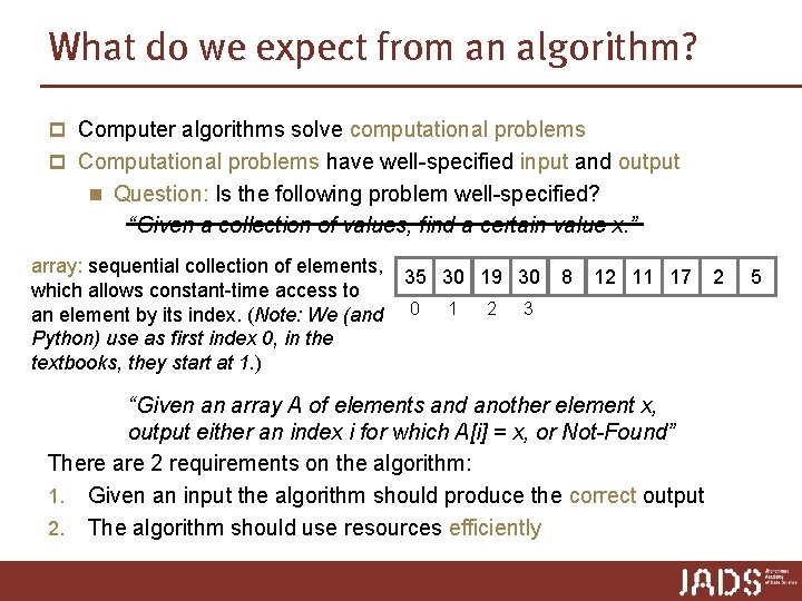
What do we expect from an algorithm? p Computer algorithms solve computational problems p Computational problems have well-specified input and output n Question: Is the following problem well-specified? “Given a collection of values, find a certain value x. ” array: sequential collection of elements, which allows constant-time access to an element by its index. (Note: We (and Python) use as first index 0, in the textbooks, they start at 1. ) 35 30 19 30 0 1 2 8 12 11 17 3 “Given an array A of elements and another element x, output either an index i for which A[i] = x, or Not-Found” There are 2 requirements on the algorithm: 1. Given an input the algorithm should produce the correct output 2. The algorithm should use resources efficiently 2 5

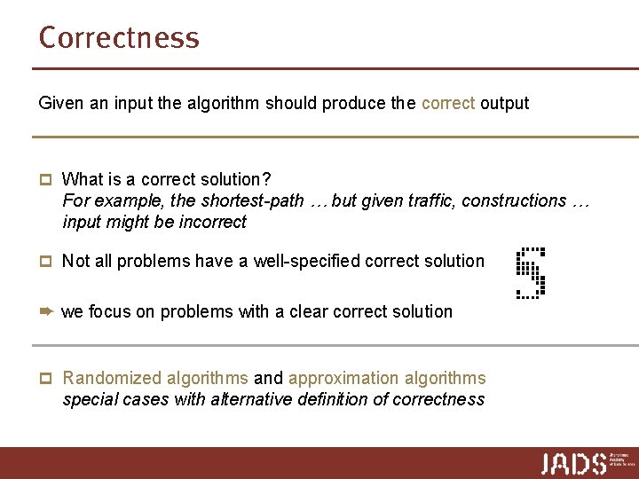
Correctness Given an input the algorithm should produce the correct output p What is a correct solution? For example, the shortest-path … but given traffic, constructions … input might be incorrect p Not all problems have a well-specified correct solution ➨ we focus on problems with a clear correct solution p Randomized algorithms and approximation algorithms special cases with alternative definition of correctness

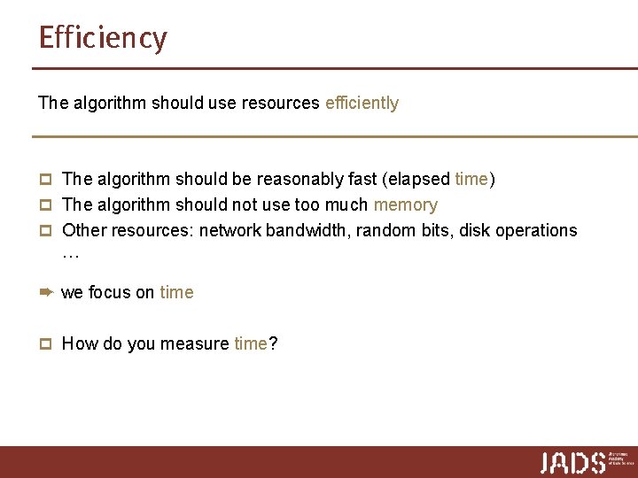
Efficiency The algorithm should use resources efficiently p The algorithm should be reasonably fast (elapsed time) p The algorithm should not use too much memory p Other resources: network bandwidth, random bits, disk operations … ➨ we focus on time p How do you measure time?

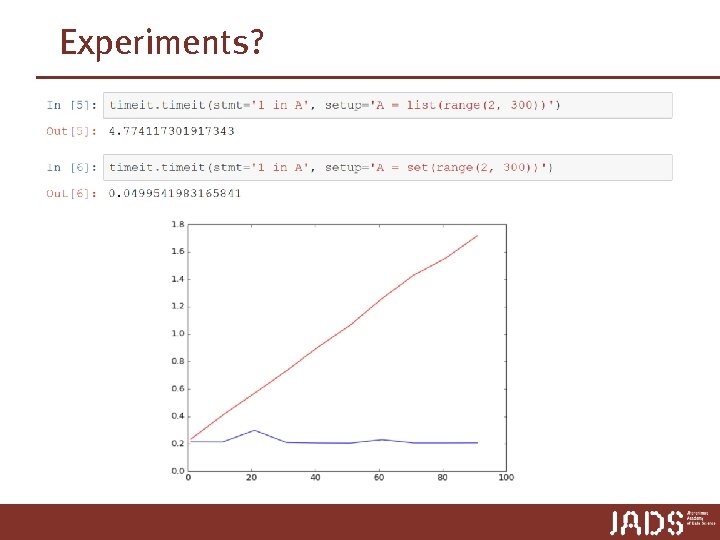
Experiments?

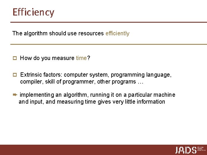
Efficiency The algorithm should use resources efficiently p How do you measure time? p Extrinsic factors: computer system, programming language, compiler, skill of programmer, other programs … ➨ implementing an algorithm, running it on a particular machine and input, and measuring time gives very little information

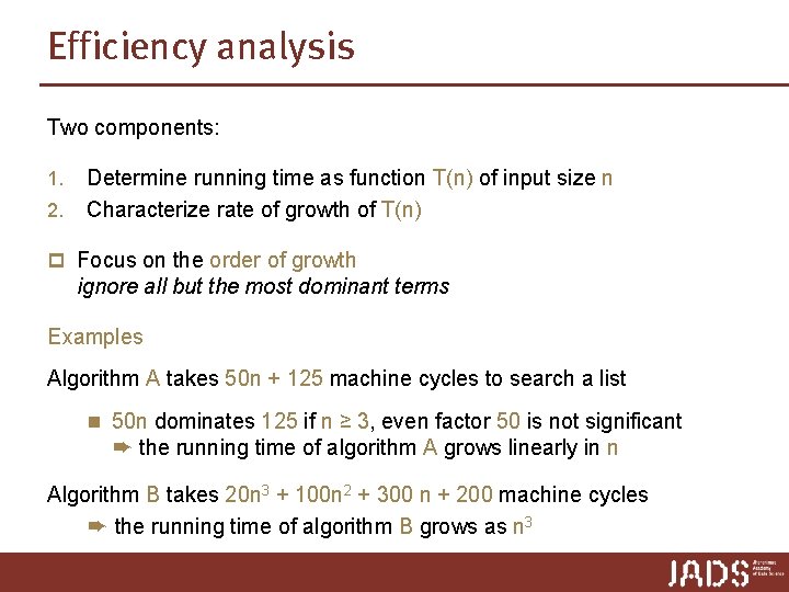
Efficiency analysis Two components: 1. 2. Determine running time as function T(n) of input size n Characterize rate of growth of T(n) p Focus on the order of growth ignore all but the most dominant terms Examples Algorithm A takes 50 n + 125 machine cycles to search a list n 50 n dominates 125 if n ≥ 3, even factor 50 is not significant ➨ the running time of algorithm A grows linearly in n Algorithm B takes 20 n 3 + 100 n 2 + 300 n + 200 machine cycles ➨ the running time of algorithm B grows as n 3

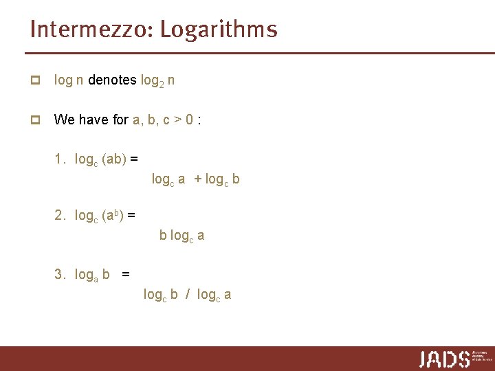
Intermezzo: Logarithms p log n denotes log 2 n p We have for a, b, c > 0 : 1. logc (ab) = logc a + logc b 2. logc (ab) = b logc a 3. loga b = logc b / logc a

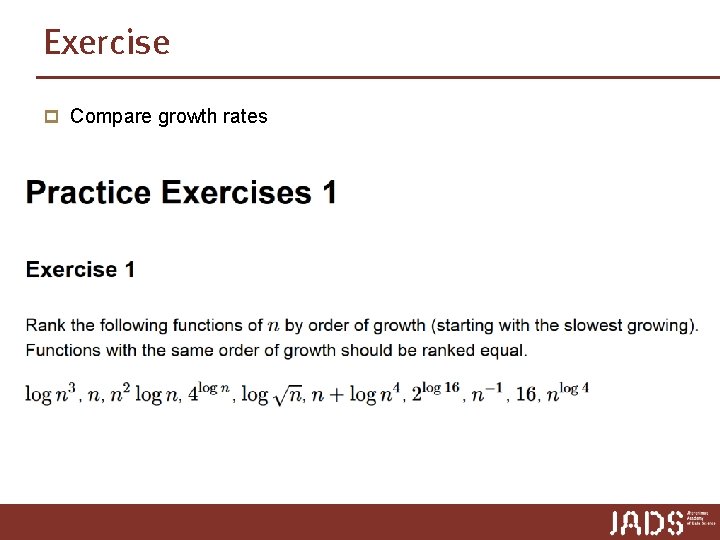
Exercise p Compare growth rates

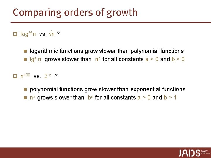
Comparing orders of growth p log 35 n vs. √n ? n logarithmic functions grow slower than polynomial functions n lga n grows slower than nb for all constants a > 0 and b > 0 p n 100 vs. 2 n ? n polynomial functions grow slower than exponential functions n na grows slower than bn for all constants a > 0 and b > 1

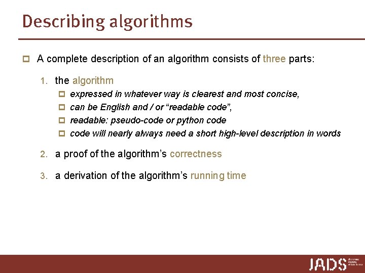
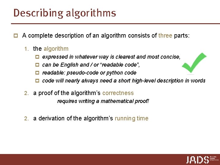
Describing algorithms p A complete description of an algorithm consists of three parts: 1. the algorithm p expressed in whatever way is clearest and most concise, p can be English and / or “readable code”, p readable: pseudo-code or python code p code will nearly always need a short high-level description in words 2. a proof of the algorithm’s correctness 3. a derivation of the algorithm’s running time

Searching

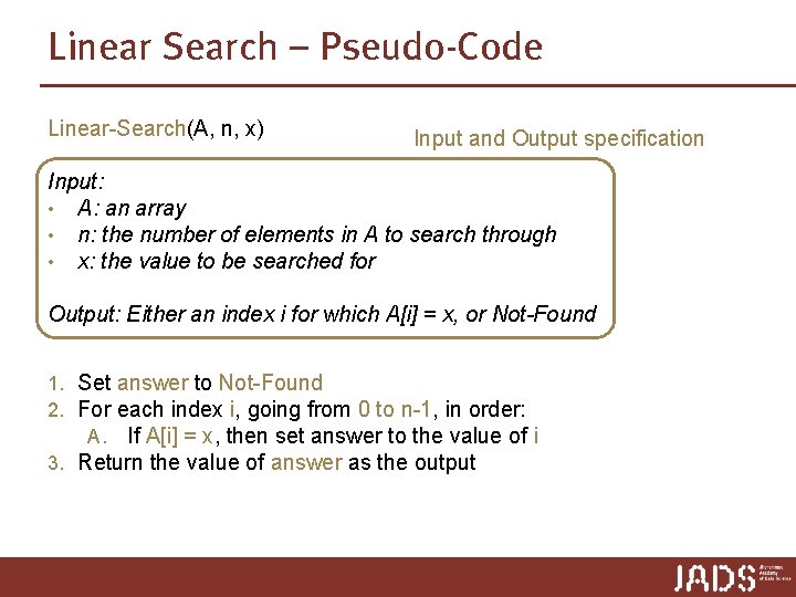
Linear Search – Pseudo-Code Linear-Search(A, n, x) Input and Output specification Input: • A: an array • n: the number of elements in A to search through • x: the value to be searched for Output: Either an index i for which A[i] = x, or Not-Found 1. Set answer to Not-Found 2. For each index i, going from 0 to n-1, in order: A. If A[i] = x, then set answer to the value of i 3. Return the value of answer as the output

Linear Search Linear-Search(A, n, x) array A[0 … n-1] 35 30 19 30 8 Input: 0 1 2 3 • A: an array • n: the number of elements in A to search through • x: the value to be searched for 12 11 17 Output: Either an index i for which A[i] = x, or Not-Found 1. Set answer to Not-Found 2. For each index i, going from 0 to n-1, in order: A. If A[i] = x, then set answer to the value of i 3. Return the value of answer as the output 2 5 n-1 A. length = n

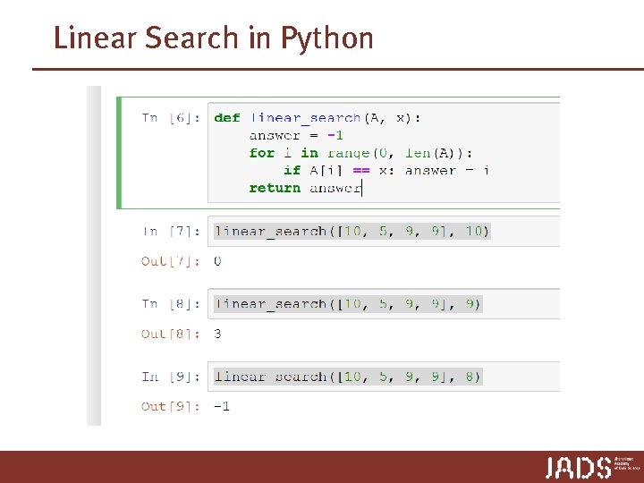
Linear Search in Python

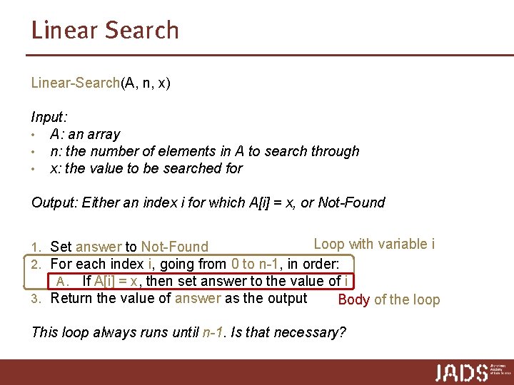
Linear Search Linear-Search(A, n, x) Input: • A: an array • n: the number of elements in A to search through • x: the value to be searched for Output: Either an index i for which A[i] = x, or Not-Found Loop with variable i 1. Set answer to Not-Found 2. For each index i, going from 0 to n-1, in order: A. If A[i] = x, then set answer to the value of i 3. Return the value of answer as the output Body of the loop This loop always runs until n-1. Is that necessary?

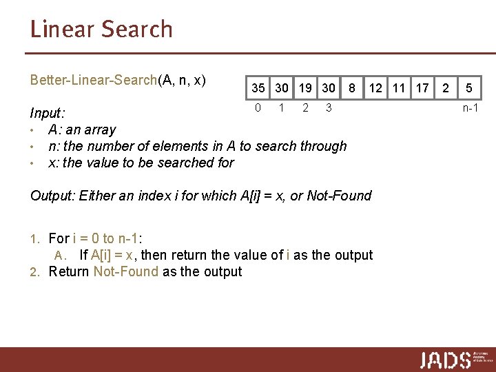
Linear Search Better-Linear-Search(A, n, x) 35 30 19 30 8 12 11 17 0 1 2 3 Input: • A: an array • n: the number of elements in A to search through • x: the value to be searched for Output: Either an index i for which A[i] = x, or Not-Found 1. For i = 0 to n-1: A. If A[i] = x, then return the value of i as the output 2. Return Not-Found as the output 2 5 n-1

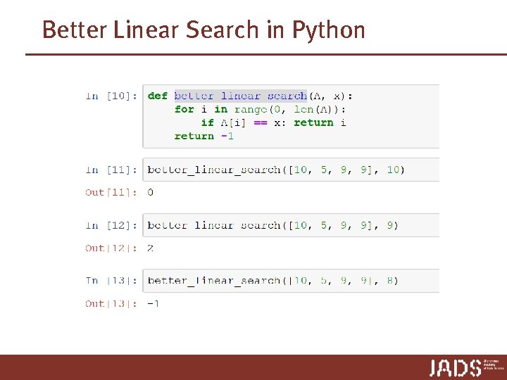
Better Linear Search in Python

Describing algorithms p A complete description of an algorithm consists of three parts: 1. the algorithm p expressed in whatever way is clearest and most concise, p can be English and / or “readable code”, p readable: pseudo-code or python code p code will nearly always need a short high-level description in words 2. a proof of the algorithm’s correctness requires writing a mathematical proof! 2. a derivation of the algorithm’s running time

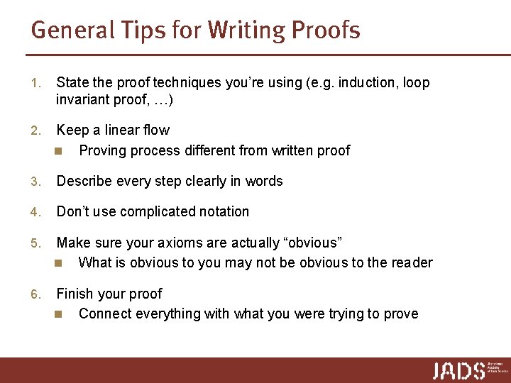
General Tips for Writing Proofs 1. State the proof techniques you’re using (e. g. induction, loop invariant proof, …) 2. Keep a linear flow n Proving process different from written proof 3. Describe every step clearly in words 4. Don’t use complicated notation 5. Make sure your axioms are actually “obvious” n What is obvious to you may not be obvious to the reader 6. Finish your proof n Connect everything with what you were trying to prove

MATHEMATICAL INDUCTION

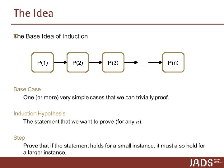
The Idea p P(1) P(2) P(3) … P(n)

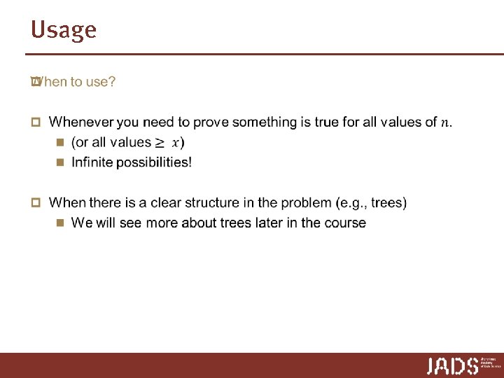
Usage p

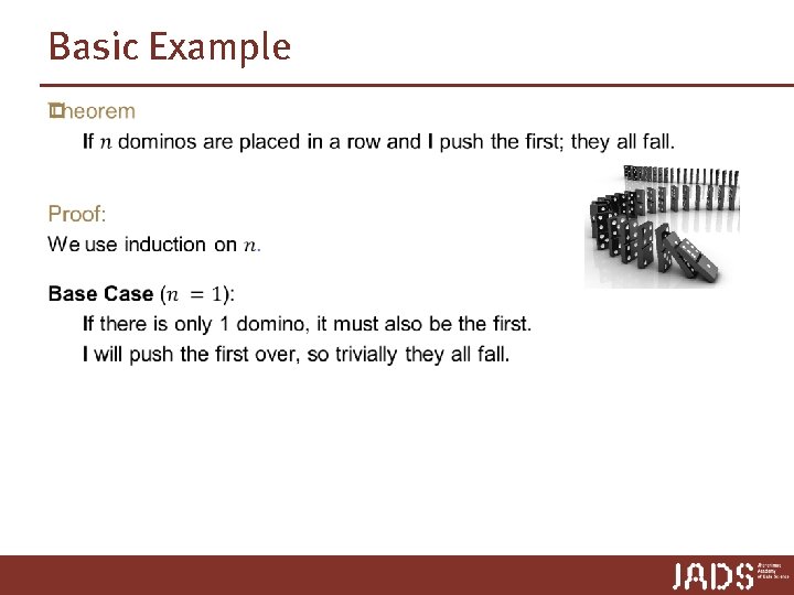
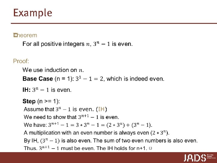
Basic Example p

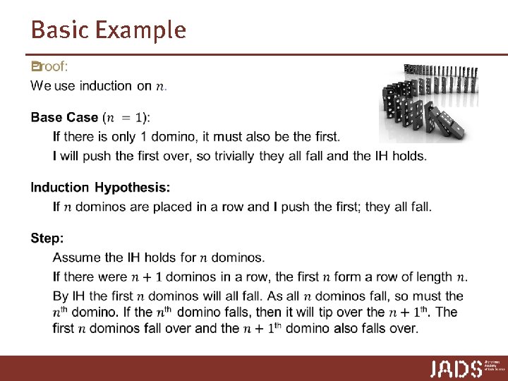
Basic Example p

Example p

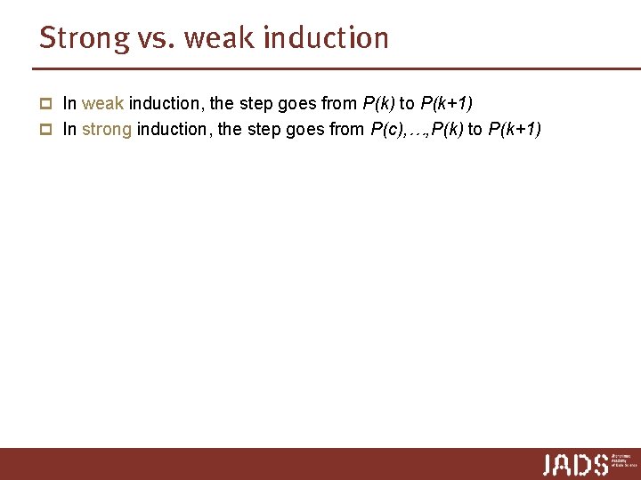
Strong vs. weak induction p In weak induction, the step goes from P(k) to P(k+1) p In strong induction, the step goes from P(c), …, P(k) to P(k+1)

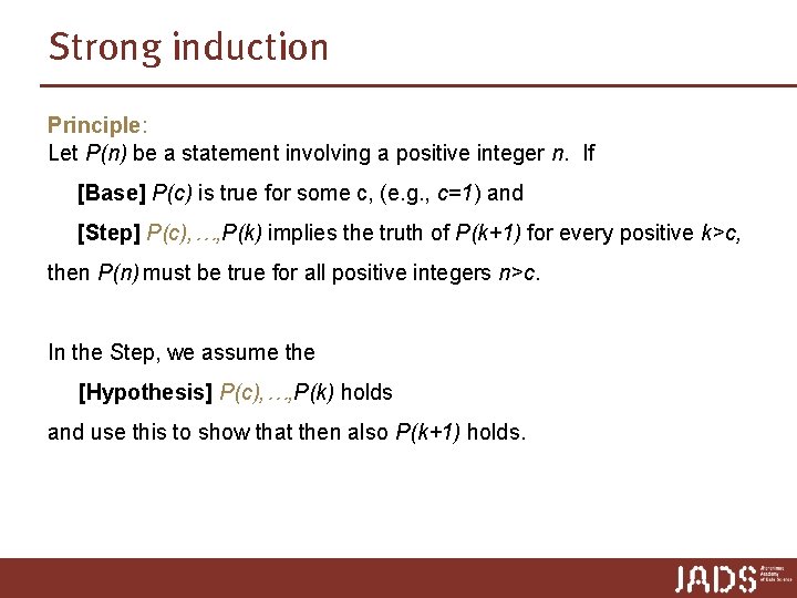
Strong induction Principle: Let P(n) be a statement involving a positive integer n. If [Base] P(c) is true for some c, (e. g. , c=1) and [Step] P(c), …, P(k) implies the truth of P(k+1) for every positive k>c, then P(n) must be true for all positive integers n>c. In the Step, we assume the [Hypothesis] P(c), …, P(k) holds and use this to show that then also P(k+1) holds.

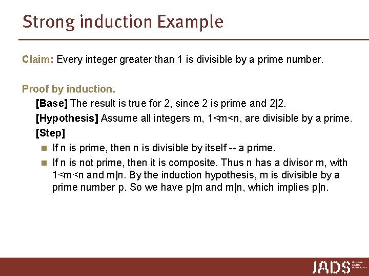
Strong induction Example Claim: Every integer greater than 1 is divisible by a prime number. Proof by induction. [Base] The result is true for 2, since 2 is prime and 2|2. [Hypothesis] Assume all integers m, 1<m<n, are divisible by a prime. [Step] n If n is prime, then n is divisible by itself -- a prime. n If n is not prime, then it is composite. Thus n has a divisor m, with 1<m<n and m|n. By the induction hypothesis, m is divisible by a prime number p. So we have p|m and m|n, which implies p|n.

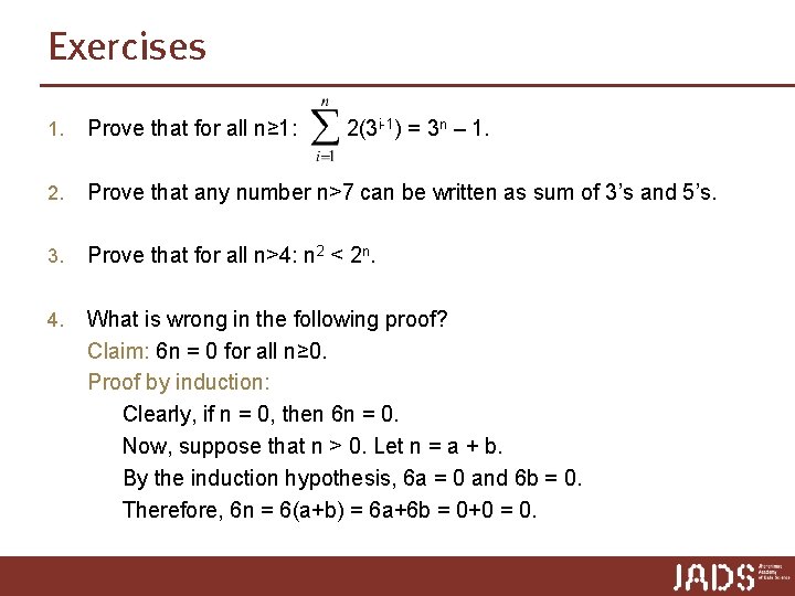
Exercises 1. Prove that for all n≥ 1: 2(3 i-1) = 3 n – 1. 2. Prove that any number n>7 can be written as sum of 3’s and 5’s. 3. Prove that for all n>4: n 2 < 2 n. 4. What is wrong in the following proof? Claim: 6 n = 0 for all n≥ 0. Proof by induction: Clearly, if n = 0, then 6 n = 0. Now, suppose that n > 0. Let n = a + b. By the induction hypothesis, 6 a = 0 and 6 b = 0. Therefore, 6 n = 6(a+b) = 6 a+6 b = 0+0 = 0.

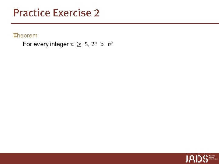
Practice Exercise 2 p

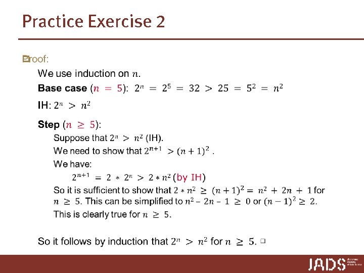
Practice Exercise 2 p

Correctness

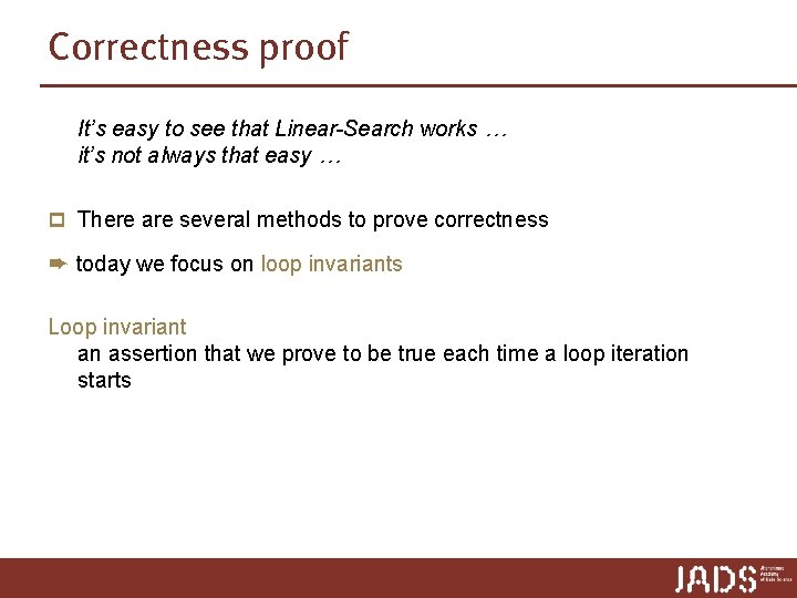
Correctness proof It’s easy to see that Linear-Search works … it’s not always that easy … p There are several methods to prove correctness ➨ today we focus on loop invariants Loop invariant an assertion that we prove to be true each time a loop iteration starts

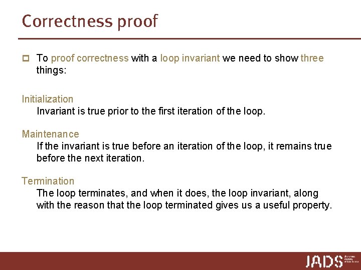
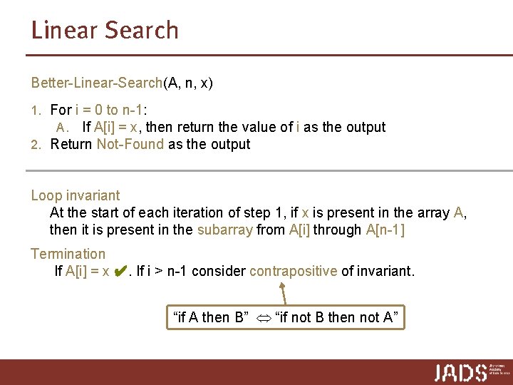
Correctness proof p To proof correctness with a loop invariant we need to show three things: Initialization Invariant is true prior to the first iteration of the loop. Maintenance If the invariant is true before an iteration of the loop, it remains true before the next iteration. Termination The loop terminates, and when it does, the loop invariant, along with the reason that the loop terminated gives us a useful property.

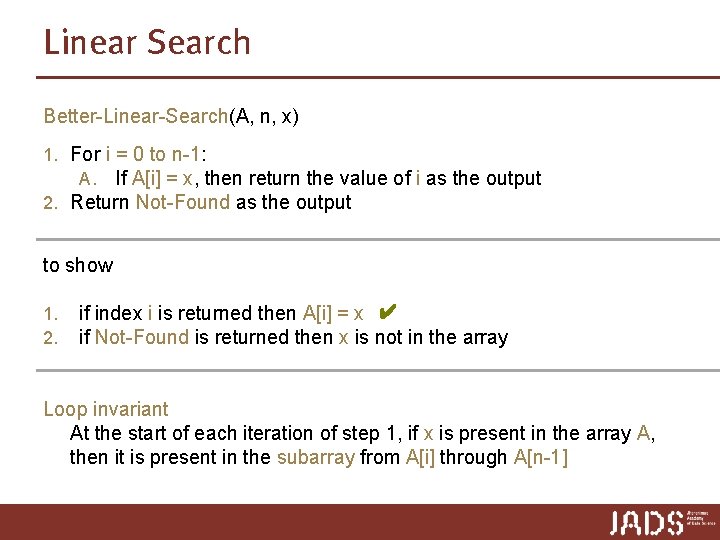
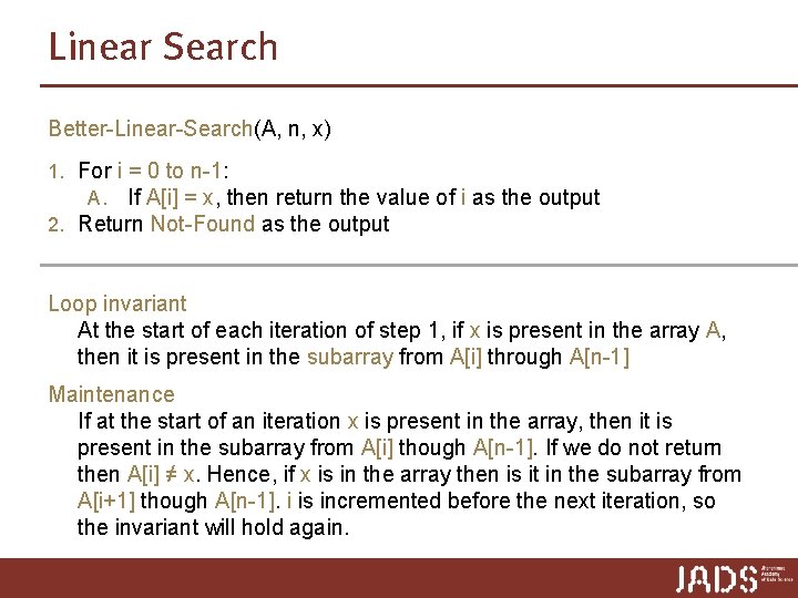
Linear Search Better-Linear-Search(A, n, x) 1. For i = 0 to n-1: A. If A[i] = x, then return the value of i as the output 2. Return Not-Found as the output to show 1. 2. if index i is returned then A[i] = x ✔ if Not-Found is returned then x is not in the array Loop invariant At the start of each iteration of step 1, if x is present in the array A, then it is present in the subarray from A[i] through A[n-1]

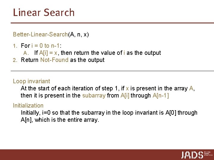
Linear Search Better-Linear-Search(A, n, x) 1. For i = 0 to n-1: A. If A[i] = x, then return the value of i as the output 2. Return Not-Found as the output Loop invariant At the start of each iteration of step 1, if x is present in the array A, then it is present in the subarray from A[i] through A[n-1] Initialization Initially, i=0 so that the subarray in the loop invariant is A[0] through A[n], which is the entire array.

Linear Search Better-Linear-Search(A, n, x) 1. For i = 0 to n-1: A. If A[i] = x, then return the value of i as the output 2. Return Not-Found as the output Loop invariant At the start of each iteration of step 1, if x is present in the array A, then it is present in the subarray from A[i] through A[n-1] Maintenance If at the start of an iteration x is present in the array, then it is present in the subarray from A[i] though A[n-1]. If we do not return then A[i] ≠ x. Hence, if x is in the array then is it in the subarray from A[i+1] though A[n-1]. i is incremented before the next iteration, so the invariant will hold again.

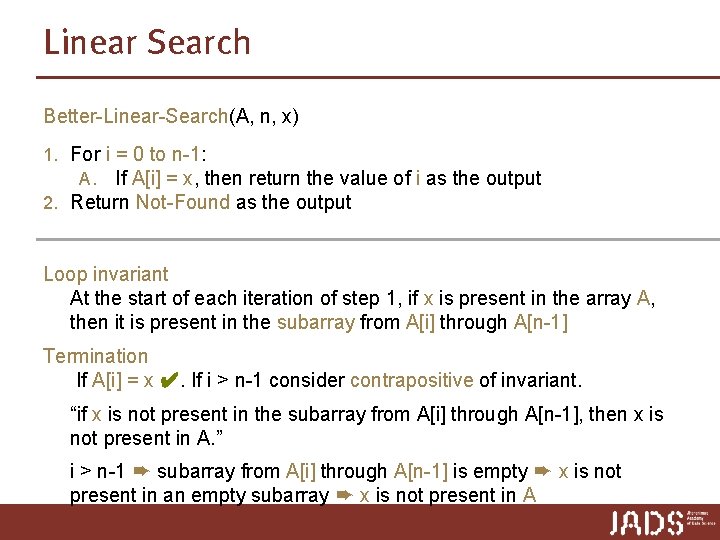
Linear Search Better-Linear-Search(A, n, x) 1. For i = 0 to n-1: A. If A[i] = x, then return the value of i as the output 2. Return Not-Found as the output Loop invariant At the start of each iteration of step 1, if x is present in the array A, then it is present in the subarray from A[i] through A[n-1] Termination If A[i] = x ✔. If i > n-1 consider contrapositive of invariant. “if A then B” “if not B then not A”

Linear Search Better-Linear-Search(A, n, x) 1. For i = 0 to n-1: A. If A[i] = x, then return the value of i as the output 2. Return Not-Found as the output Loop invariant At the start of each iteration of step 1, if x is present in the array A, then it is present in the subarray from A[i] through A[n-1] Termination If A[i] = x ✔. If i > n-1 consider contrapositive of invariant. “if x is not present in the subarray from A[i] through A[n-1], then x is not present in A. ” i > n-1 ➨ subarray from A[i] through A[n-1] is empty ➨ x is not present in an empty subarray ➨ x is not present in A

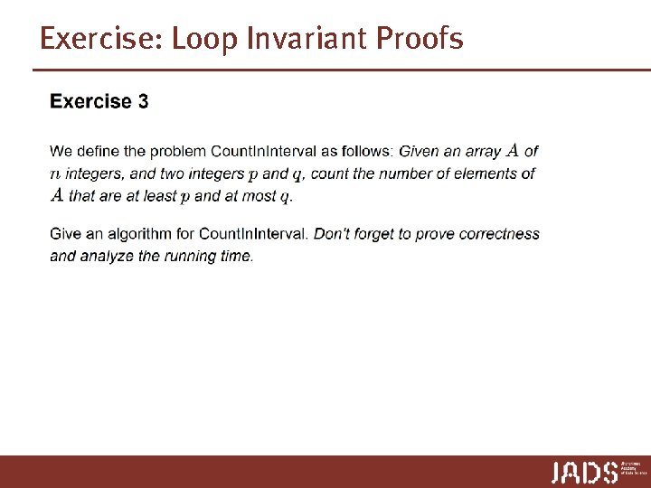
Exercise: Loop Invariant Proofs

Recap and preview Today p Describing algorithms p Efficiency Analysis (informal) p Linear Search p Mathematical induction p Correctness proofs via loop invariants Next lecture p Efficiency analysis (formal) p Binary Search p Recursive algorithms