Data Structure The Big Picture Chapter 1 1

Lecture 1 2

Introduction • A data structure is a data organization, management, and storage format that enables efficient access and modification. • More precisely, a data structure is a collection of: • Data values, • The relationships among them, • And the functions or operations that can be applied to the data. 3

Introduction • Suppose we need to answer the following Questions: • How many cities with more than 250, 000 people lie within 500 miles of Dallas, Texas? • How many people in my company make over $100, 000 per year? • Can we connect all of our telephone customers with less than 1, 000 miles of cable? • To answer above questions, We must organize data in a way that allows us to find the answers in time to satisfy our needs. 4

Introduction • The primary purpose of most computer programs is not only to perform calculations, but also to store and retrieve information usually as fast as possible. • For this reason, the study of data structures and the algorithms that manipulate them is at the heart of computer science. helping you to understand how to structure data to support efficient processing. 5

Atomic and Composite Data Type • Atomic or primitive type A data type whose elements are single, non decomposable data items (cannot be broken into parts) • Composite type A data type whose elements are composed of multiple data items. (ex: take tow integers (simple elements) x, y to form a point (x, y) 6

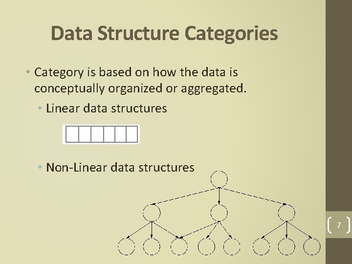
Data Structure Categories • Category is based on how the data is conceptually organized or aggregated. • Linear data structures • Non-Linear data structures 7

Linear Data Structures • Data structure where data elements are arranged sequentially or linearly. • Linear data structures are easy to implement because computer memory is arranged in a linear way. • Examples on Linear data structures : array, unordered list, stack, queue, etc. 8

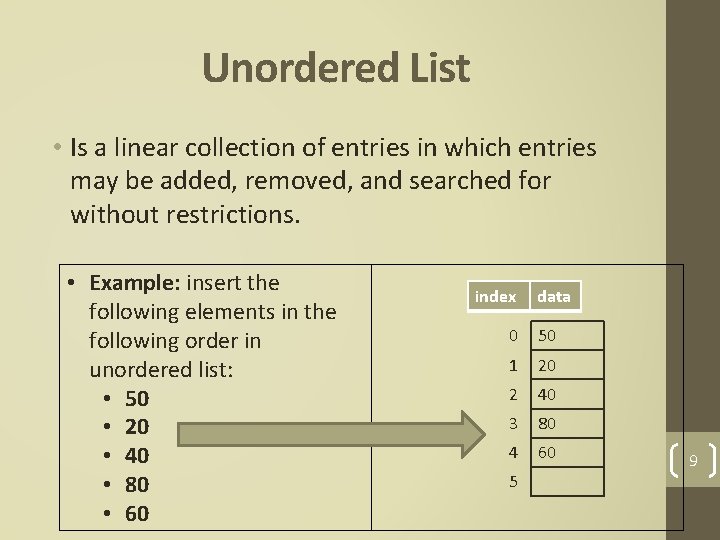
Unordered List • Is a linear collection of entries in which entries may be added, removed, and searched for without restrictions. • Example: insert the following elements in the following order in unordered list: • 50 • 20 • 40 • 80 • 60 index data 0 50 1 20 2 40 3 80 4 60 5 9

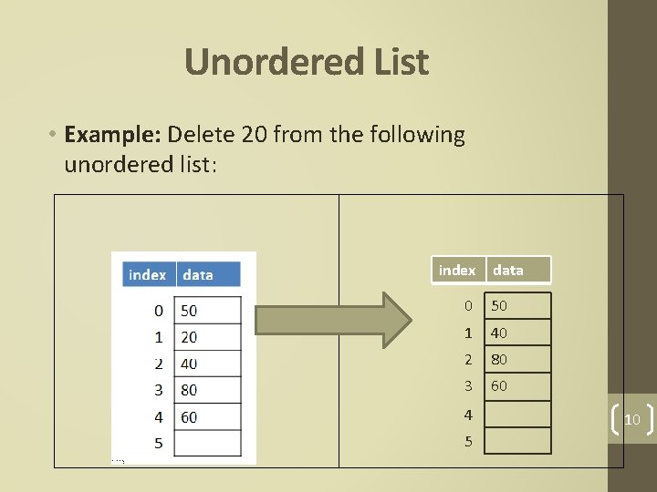
Unordered List • Example: Delete 20 from the following unordered list: index data 0 50 1 40 2 80 3 60 4 5 10

Ordered List • Is a linear collection of sorted (from smallest to largest or from largest to smallest )in which entries may be added, removed, and searched for with only one restriction is that the elements should remains sorted. 11

Ordered List • Example: insert the following elements in the following order in ordered list: • • • 50 20 40 80 60 12

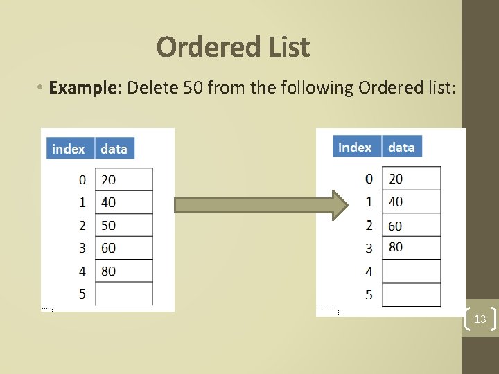
Ordered List • Example: Delete 50 from the following Ordered list: 13

Exercise 1 A. Insert the following elements in the following order in unordered list: • 70 • 110 • 30 • 55 • 46 B. Delete 110 from the result unordered list in part A. 14

Exercise 2 A. Insert the following elements in the following order in ordered list: • 70 • 110 • 30 • 55 • 46 B. Delete 110 from the result ordered list in part A. 15

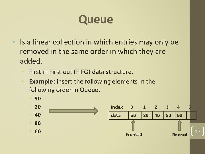
Queue • Is a linear collection in which entries may only be removed in the same order in which they are added. • First in First out (FIFO) data structure. • Example: insert the following elements in the following order in Queue: • • • 50 20 40 80 60 index 0 1 2 3 4 data 50 20 40 80 60 Front=0 Rear=4 5 16

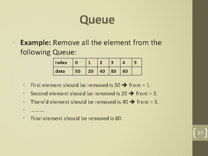
Queue • Example: Remove all the element from the following Queue: • • • index 0 1 2 3 4 data 50 20 40 80 60 5 First element should be removed is 50 front = 1. Second element should be removed is 20 front = 2. There'd element should be removed is 40 front = 3. ………. Final element should be removed is 60. 17

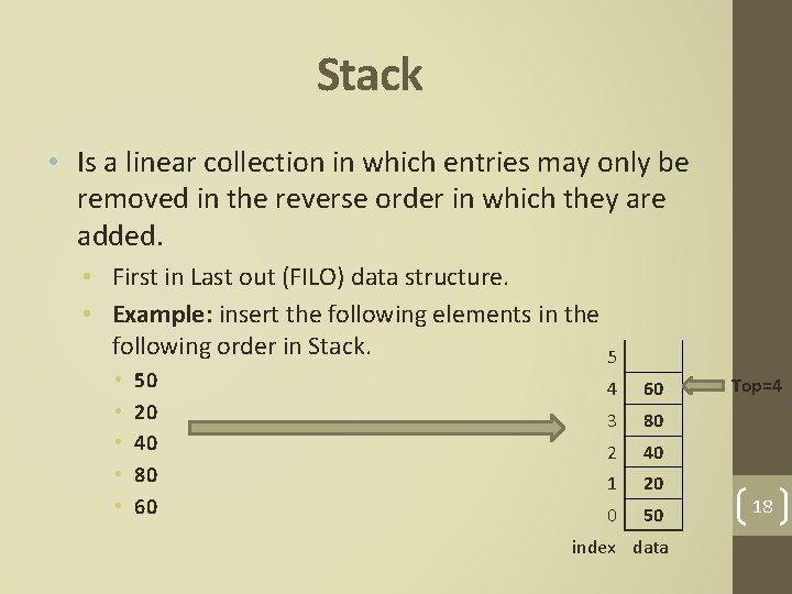
Stack • Is a linear collection in which entries may only be removed in the reverse order in which they are added. • First in Last out (FILO) data structure. • Example: insert the following elements in the following order in Stack. 5 • • • 50 20 40 80 60 4 60 3 80 2 40 1 20 0 50 index data Top=4 18

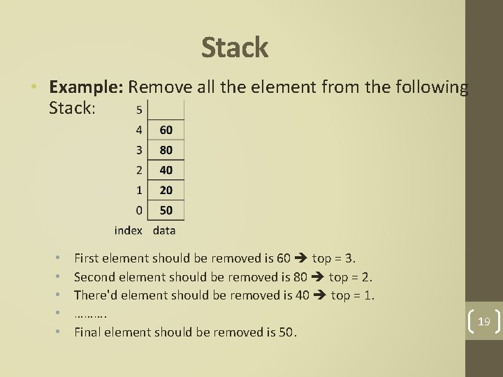
Stack • Example: Remove all the element from the following Stack: • • • First element should be removed is 60 top = 3. Second element should be removed is 80 top = 2. There'd element should be removed is 40 top = 1. ………. Final element should be removed is 50. 19

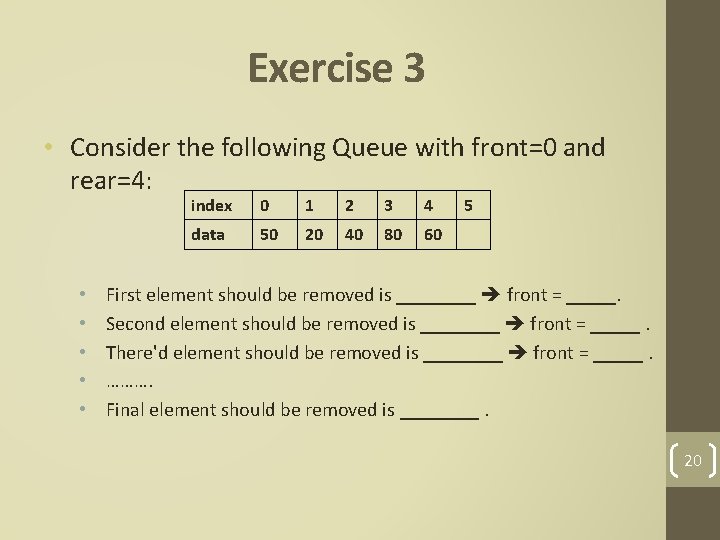
Exercise 3 • Consider the following Queue with front=0 and rear=4: • • • index 0 1 2 3 4 data 50 20 40 80 60 5 First element should be removed is ____ front = _____. Second element should be removed is ____ front = _____. There'd element should be removed is ____ front = _____. ………. Final element should be removed is ____. 20

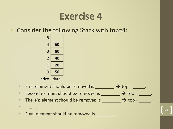
Exercise 4 • Consider the following Stack with top=4: • • • First element should be removed is ____ top = _____. Second element should be removed is ____ top = _____. There'd element should be removed is ____ top = _____. ………. Final element should be removed is ____. 21

Non-Linear Data Structures • Data structures where data elements are not arranged sequentially or linearly. • Non-linear data structures are not easy to implement in comparison to linear data structure. • Examples on Non-Linear data structures : trees and graphs. 22

Trees • A nonlinear data structure with a unique starting node (the root). • Root: The top node of a tree structure; a node with no parent • Each node is capable of having many child nodes • A unique path exists from the root to every other node. • Are useful for representing hierarchical relationships among data items. 23

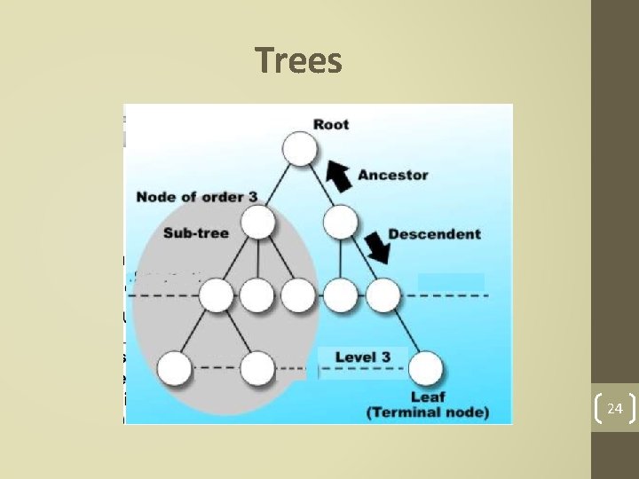
Trees 24

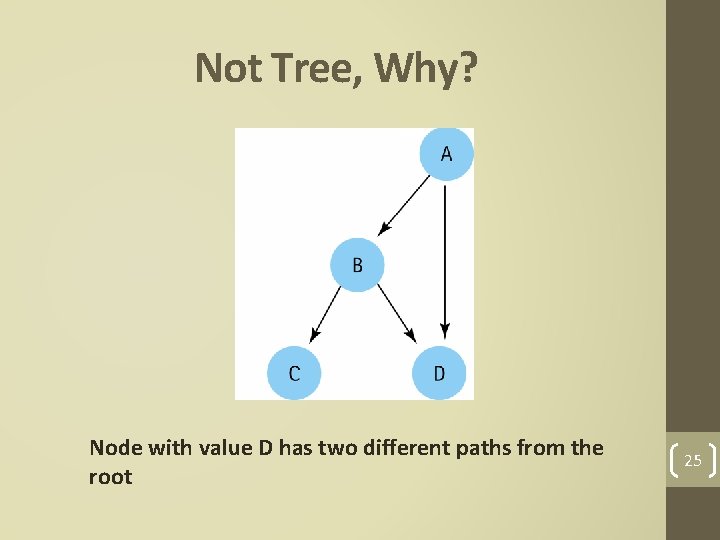
Not Tree, Why? Node with value D has two different paths from the root 25

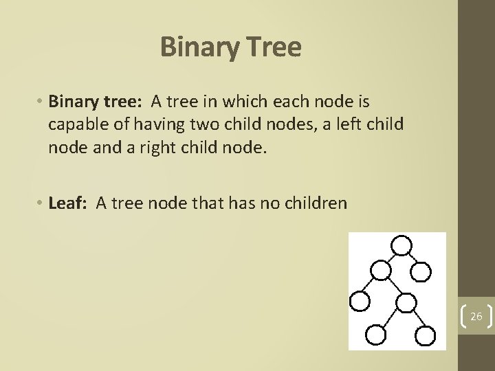
Binary Tree • Binary tree: A tree in which each node is capable of having two child nodes, a left child node and a right child node. • Leaf: A tree node that has no children 26

Lecture 2 27

Binary Search Tree • A binary tree in which the key value in any node is greater than the key value in its left child any of its descendants (the nodes in the left subtree) and less than the key value in its right child any of its descendants (the nodes in the right subtree) 28

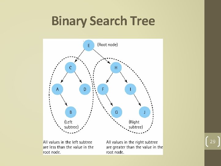
Binary Search Tree 29

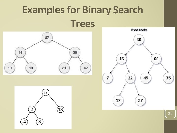
Examples for Binary Search Trees 30

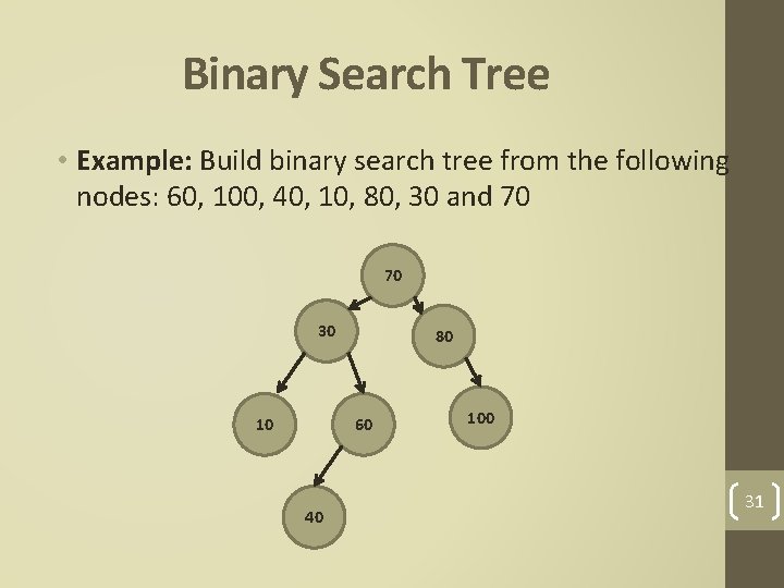
Binary Search Tree • Example: Build binary search tree from the following nodes: 60, 100, 40, 10, 80, 30 and 70 70 30 10 80 60 40 100 31

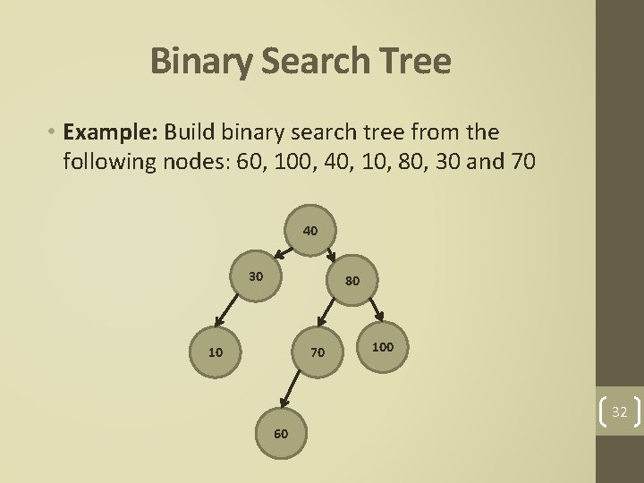
Binary Search Tree • Example: Build binary search tree from the following nodes: 60, 100, 40, 10, 80, 30 and 70 40 30 80 10 70 100 32 60

Exercise 5 • Build binary search tree from the following nodes: 10, 100, 50, 40, 88, 70, 60, 15 and 99 33

Priority Queue • A priority queue is a special type of queue in which each element is associated with a priority and is served according to its priority. • If elements with the same priority occur, they are served according to their order in the queue. 34

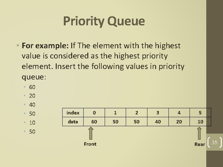
Priority Queue • For example: If The element with the highest value is considered as the highest priority element. Insert the following values in priority queue: • • • 60 20 40 50 10 50 index 0 1 2 3 4 5 data 60 50 50 40 20 10 Front Rear 35

Exercise 6 • Insert the following values in priority queue: • • • 5 30 80 10 60 10 36

Heap • Heap is complete binary tree data structure which has two types: • Max heap: for any given node C, if P is any text node in each of node C subtrees , then the key (the value) of P is less than or equal to the key of C. • Min heap: for any given node C, if P is any node in each of node C left subtrees, then the key (the value) of P is less than or equal to the key of C. . 37

Complete Binary Tree • A complete binary tree is one in which every level but the last must have the maximum number of nodes possible at that level. • The last level may have fewer than the maximum possible nodes, but they should be arranged from left to right without any empty spots. 38

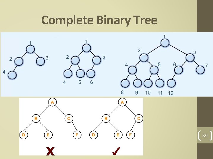
Complete Binary Tree 39

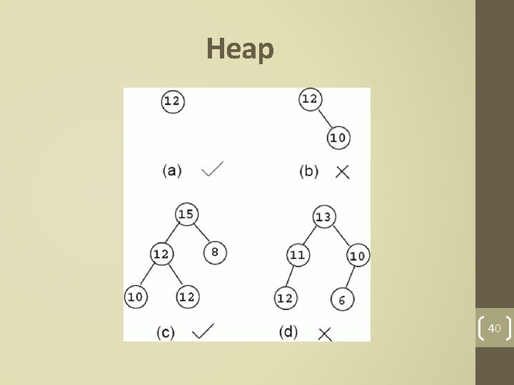
Heap 40

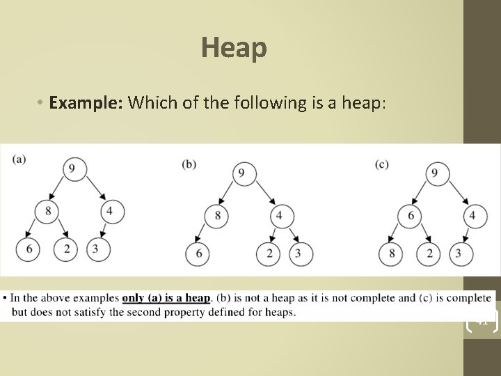
Heap • Example: Which of the following is a heap: 41

Exercise 7 • Construct a heap using the following values: • • 22 10 100 90 44 60 80 42

Hash Table • Hash table: Term used to describe the data structure used to store and retrieve elements using hashing. • Hashing: The technique for ordering and accessing elements in a list in a relatively constant amount of time by manipulating the key to identify its location in the list. • Hash Functions: A function used to manipulate the key of an element in a list to identify its location in the list 43

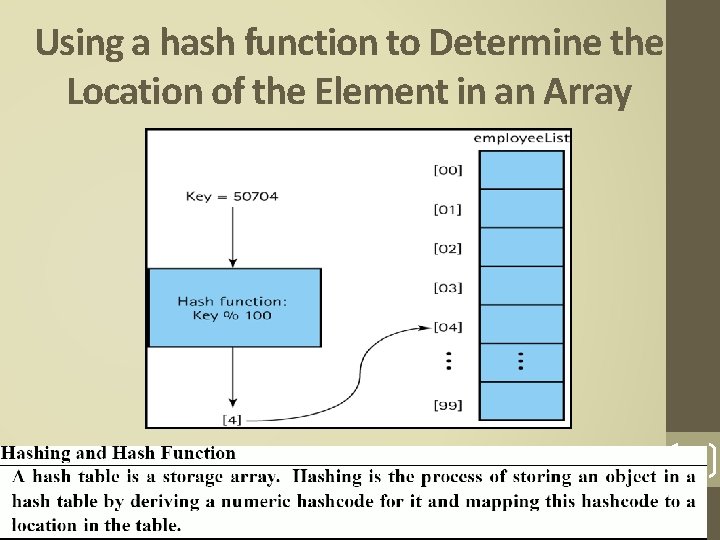
Using a hash function to Determine the Location of the Element in an Array 44

Graphs • Graph: A data structure that consists of a set of nodes and a set of edges that relate the nodes to each other • Edge (arc): representing a connection between two nodes in a graph. • Two kinds of graphs: • Undirected graph: A graph in which the edges have no direction. • Directed graph (digraph): A graph in which each edge is directed from one vertex to another (or the same) vertex. 45

Graphs • A general tree is a special kind of graph. • Graphs may be used to model: • Computer networks, • Airline routes. • As abstract relationships such as course prerequisite structures, etc. . 46

Graphs • Adjacent nodes: Two nodes in a graph that are connected by an edge. • Path: A sequence of nodes that connects two nodes in a graph. • Complete graph: A graph in which every node is directly connected to every other node. 47 • Weighted graph: A graph in which each edge carries a value.

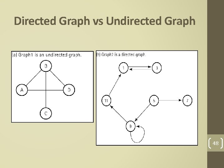
Directed Graph vs Undirected Graph 48

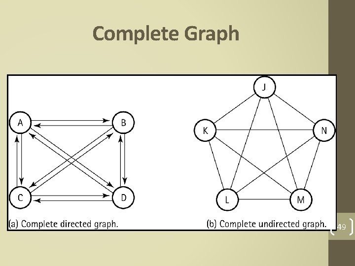
Complete Graph 49

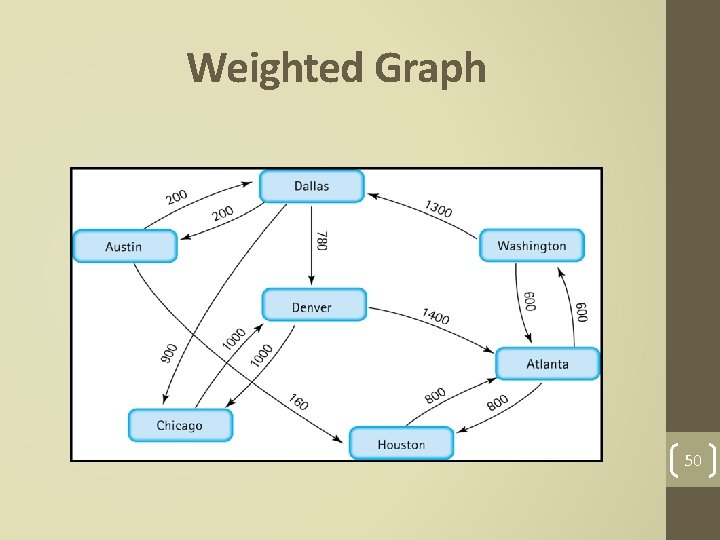
Weighted Graph 50

Lecture 3 51

Data Type • Meaningful data is organized into: • Primitive data types such as integer, real, and Boolean. • And into more complex data structures such as arrays and binary trees. • So the idea of a data type includes: • A specification of the possible values of that type. • The operations that can be performed on those values. 52

Abstract Data Type (ADT) • A data type whose properties (domain and operations) are specified independently of any particular implementation. • The definition of ADT only mentions what operations are to be performed but not how these operations will be implemented. 53

Abstract Data Type (ADT) • It does not specify how data will be organized in memory and what algorithms will be used for implementing the operations. • It is called “abstract” because it gives an implementation-independent view. • The process of providing only the essentials and hiding the details is known as abstraction. • The primitive data types is abstract data types. 54

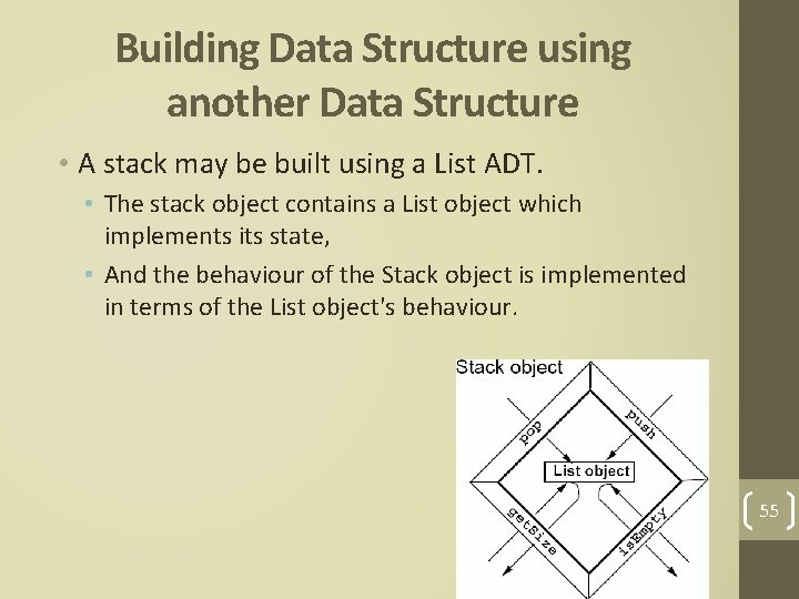
Building Data Structure using another Data Structure • A stack may be built using a List ADT. • The stack object contains a List object which implements its state, • And the behaviour of the Stack object is implemented in terms of the List object's behaviour. 55

Choosing the Right Data Structure for Specific Problem • The operations that is supported by a data structure is one factor to consider when choosing between several available data structures. • Example: • Implementing a printing job storage for a printer: • requires a queue data structure. • Maintains a collection of entries in no particular order. • requires an unordered list data structure. 56

Choosing the Right Data Structure for Specific Problem • The efficiency of the data structures is another factor to consider when choosing between several available data structures : • How much space does the data structure occupy? • What are the running times of the operation in its interface? 57

Choosing the Right Data Structure for Specific Problem • The running time of each operation in the interface: • A data structure with the best interface with the best fit may not necessarily be the best overall fit, if the running times of its operations are not up to the mark. 58

Choosing the Right Data Structure for Specific Problem • When we have more than one data structure implementation whose interfaces satisfy our requirements, we may have to select one based on comparing the running times of the interface operations. • Time is traded off for space, • i. e. more space is consumed to increase speed, or a reduction in speed is traded for a reduction in the space consumption. 59

Time complexity • Use of time complexity makes it easy to estimate the running time of a program. • Complexity can be viewed as the maximum number of primitive operations that a program may execute. • Regular operations are single additions, multiplications, assignments etc. • We may leave some operations uncounted and concentrate on those that are performed the largest number of times. • Such operations are referred to as dominant. 60

Big-O notation complexity • The complexity specifies the order of magnitude within which the program will perform its operations. • In the case of O(n), the program may perform (cn) operations, where c is a constant. • In other words, when calculating the complexity we omit constants: • i. e. regardless of whether the loop is executed (20 x n) times or (n/ 5) times, we still have a complexity of O(n), even though the running time of the program may vary. 61

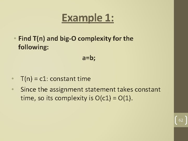
Example 1: • Find T(n) and big-O complexity for the following: a=b; • T(n) = c 1: constant time • Since the assignment statement takes constant time, so its complexity is O(c 1) = O(1). 62

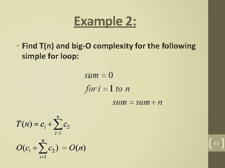
Example 2: • Find T(n) and big-O complexity for the following simple for loop: 63

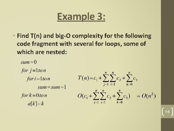
Example 3: • Find T(n) and big-O complexity for the following code fragment with several for loops, some of which are nested: 64

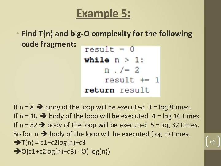
Example 5: • Find T(n) and big-O complexity for the following code fragment: If n = 8 body of the loop will be executed 3 = log 8 times. If n = 16 body of the loop will be executed 4 = log 16 times. If n = 32 body of the loop will be executed 5 = log 32 times. So for n body of the loop will be executed (log n) times. T(n) = c 1+c 2 log(n)+c 3 O(c 1+c 2 log(n)+c 3) =O( log(n)) 65

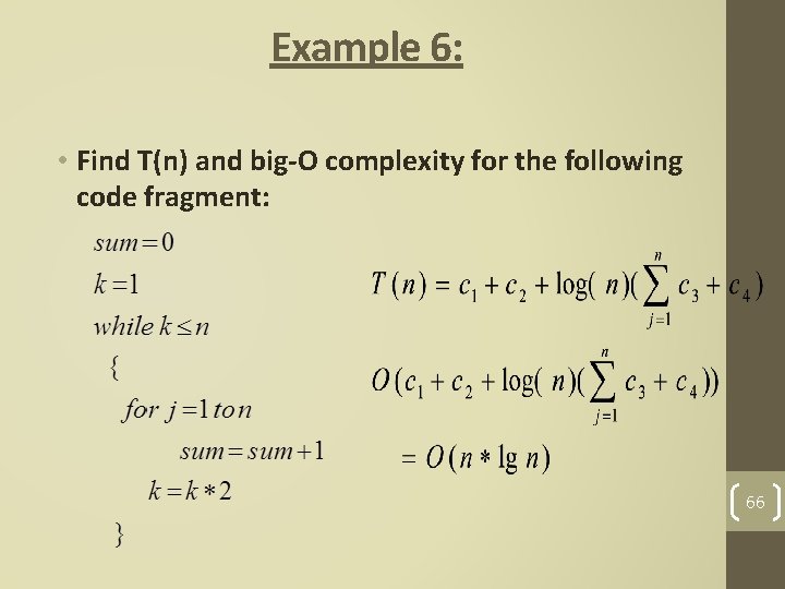
Example 6: • Find T(n) and big-O complexity for the following code fragment: 66

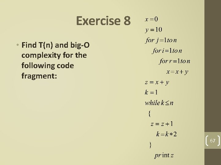
Exercise 8 • Find T(n) and big-O complexity for the following code fragment: 67

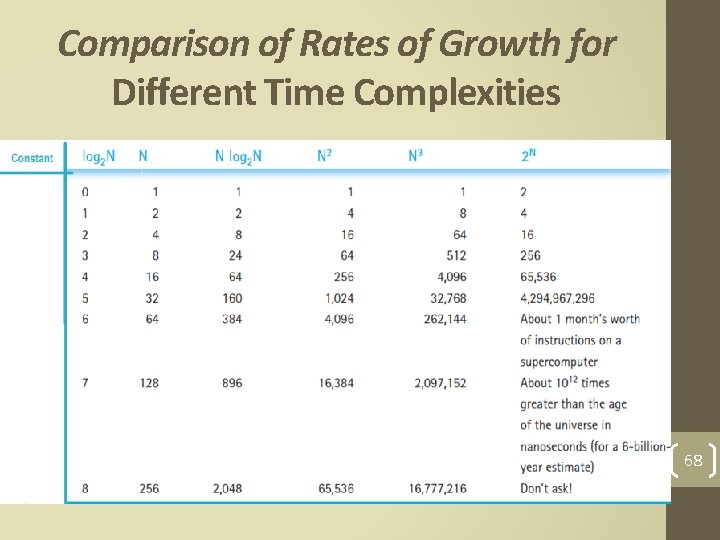
Comparison of Rates of Growth for Different Time Complexities 68

Exercise 9 • If we can use any one of the following data structures to solve a problem and the only difference between the following data structures is the implementation of a function (get. Size) where the complexity time for this function for each data structure is as following: • T(n) for get. Size in first data structure is = 20 n+30. • T(n) for get. Size in second data structure is = 2 n 2+3 n+50 • T(n) for get. Size in last data structure is = 4 n+3 nlog(n)+50 log(n) • Use big-O complexity to determine which data structure should we use? and why? 69

Summary • A data structure is a data organization, management, and storage format. • Data type is either atomic or composite. • Data structure category is based on how the data is conceptually organized or aggregated(linear or nonlinear) • Unordered list Is a linear collection of entries in which entries may be added, removed, and searched for without restrictions. 70

Summary • Ordered list Is a linear collection of sorted in which entries may be added, removed, and searched for with only one restriction is that the elements should remains sorted • Queue Is a linear collection in which entries may only be removed in the same order in which they are added. • Stack Is a linear collection in which entries may only be removed in the reverse order in which they are added. • Tree is a nonlinear data structure with a unique starting node and a unique path exists from the root to every other node. 71

Summary • Binary tree is A tree in which each node is capable of having two child nodes, a left child node and a right child node. • Binary search tree is a binary tree in which the key value in any node is greater than the key value in its left child any of its descendants and less than the key value in its right child any of its descendants • Priority queue is a special type of queue in which each element is associated with a priority and is served according to its priority. 72

Summary • Max heap is complete binary tree where for any given node C, if P is any node in each of node C subtrees , then the key (the value) of P is less than or equal to the key of C. • Min heap is complete binary tree where for any given node C, if P is any node in each of node C subtrees , then the key (the value) of P is greater than or equal to the key of C. • Complete binary tree is one in which has no empty spot before the last node. • Hash table is data structure used to store and retrieve elements using hash function. 73

Summary • Abstract Data Type (ADT) is A data type whose properties (domain and operations) are specified independently of any particular implementation. • The operations that is supported by a data structure is one factor to consider when choosing between several available data structures. • When we have more than one data structure implementation whose interfaces satisfy our requirements, we may have to select one based on comparing the running times of the interface operations. 74

Summary • Use of time complexity makes it easy to estimate the running time of a program. • Big-O notation complexity is The complexity specifies the order of magnitude within which the program will perform its operations. 75

References • Data Structures Outside-In With Java, Sesh Venugopal, Prentice Hall. • https: //codility. com/media/train/1 -Time. Complexity. pdf 76