Data Stream Mining Tore Risch Dept of information

Data Stream Mining Tore Risch Dept. of information technology Uppsala University Sweden 2014 -05 -14

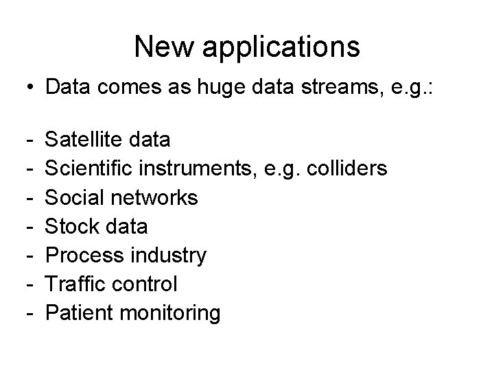
New applications • Data comes as huge data streams, e. g. : - Satellite data Scientific instruments, e. g. colliders Social networks Stock data Process industry Traffic control Patient monitoring

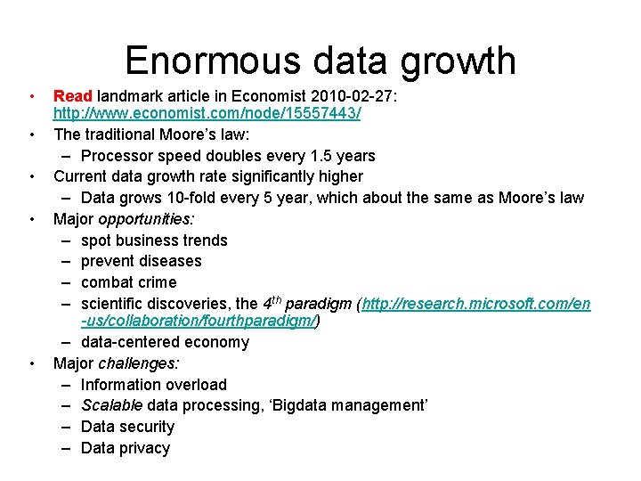
Enormous data growth • • • Read landmark article in Economist 2010 -02 -27: http: //www. economist. com/node/15557443/ The traditional Moore’s law: – Processor speed doubles every 1. 5 years Current data growth rate significantly higher – Data grows 10 -fold every 5 year, which about the same as Moore’s law Major opportunities: – spot business trends – prevent diseases – combat crime – scientific discoveries, the 4 th paradigm (http: //research. microsoft. com/en -us/collaboration/fourthparadigm/) – data-centered economy Major challenges: – Information overload – Scalable data processing, ‘Bigdata management’ – Data security – Data privacy

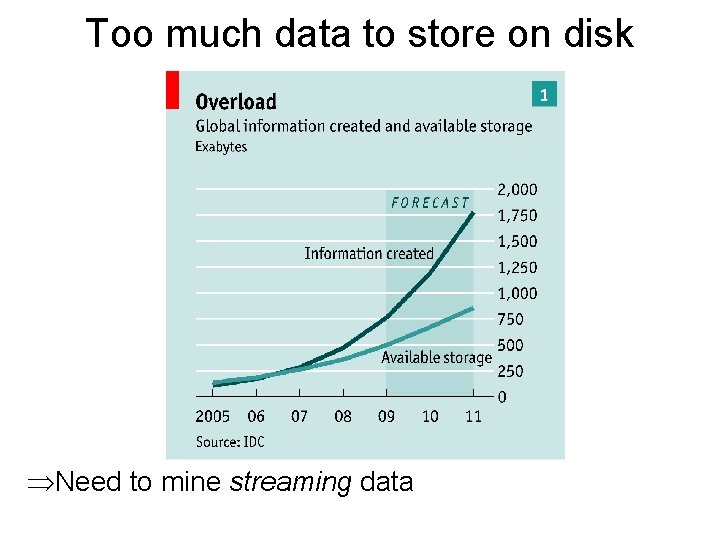
Too much data to store on disk ÞNeed to mine streaming data

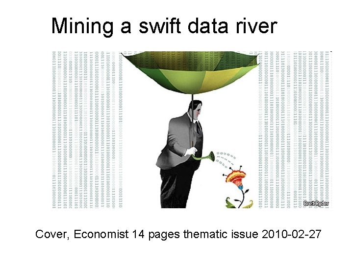
Mining a swift data river Cover, Economist 14 pages thematic issue 2010 -02 -27

Mining streams vs. databases • Data streams dynamic and infinite in size – – Data is continuously generated and changing Live streams may have no upper limit A live stream, can be read only once (‘Just One Look’) The stream rate may be very high • Traditional data mining does not work for streaming data: – Regular data mining based on finite data collections stored in files or databases – Regular data mining done in batch: • read (access) data in collection several times • analyze accessed data • store results in database (or file) – For example, store for each data object what cluster it belongs to

Data stream mining vs. traditional data mining • Live streams grow continuously – The system cannot read streams many times as with traditional data mining • Live streams mining must be done on-line – Not traditional batch processing • Live streams require main memory processing – To keep up with very high data flow rates (speed) • Live streams must be mined with limited memory – Not load-analyze as traditional data mining – Iterative processing of statistics • Live streams must keep up with very high data flow volumes – Approximate mining algorithms – Parallel on-line computations

Streams vs. regular data • Data stream mining requires iterative aggregation: – Read data tuples iteratively from input stream(s) • E. g. measured values • Do not store read data in database – Analyze read tuples incrementally – Keep partial results in main memory • E. g. sum and count – Continuosly emit incremental analyzed resuls • E. g. running average by dividing sum with count • Result of data stream mining is derived stream – Continuously produced by emit – Can be stored as continuously changing database

Streams vs. regular data • Stream processing should keep up with data flow – Make computations so fast that they keep up with the flow (on average) – Should not be catastrophic if if miner cannot keep up with the flow: • Drop input data values • Use approximate computations such as sampling • Asynchronous logging in files often possible – At least of processed (reduced) streaming data – At least during limited time (log files)

Requirements for Stream Mining • Single scan of data, – because of very large or infinite size of streams. – because it may be impossible or very expensive to reread the stream for the computation • Limited memory and CPU usage – because the processing should be done in main memory despite the very large stream volume • Compact continuously evolving representation of mined data – It is not possible to store the mined data in database as with traditional data mining – A compact main memory representation of mined data needed

Requirements for Stream Mining • Allow for continuous evolution of mined data – Traditional batch mining static mined data – Continuous mining makes mined data into a stream too =>Concept drift • Often mining over different kinds of windows of streams – E. g. sliding or tumbling windows – Windows of limited size – Often only statistics summaries needed (synopses, sketches)

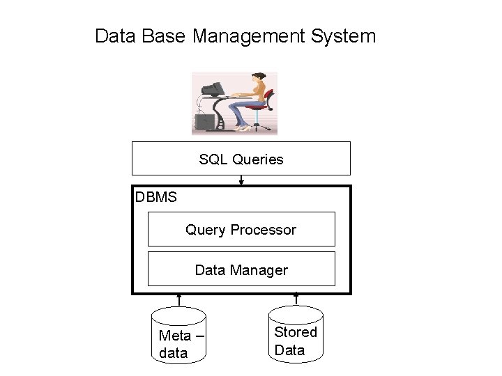
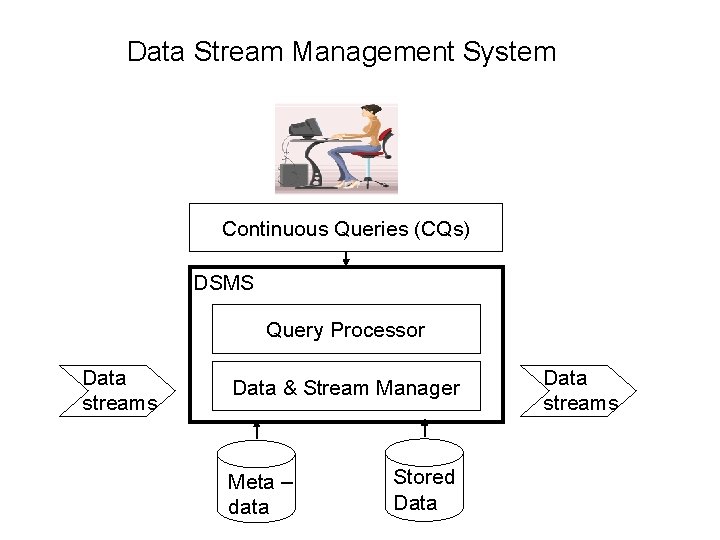
Data Stream Management Systems (DSMS) • Data. Base Management System (DBMS) – General purpose software to handle large volume persistent data (usually on disk) – Important tool for traditional datamining • Data Stream Management System (DSMS) – General purpose software to handle large volume data streams (often transient data) – Important tool for data stream mining

Data Base Management System SQL Queries DBMS Query Processor Data Manager Meta – data Stored Data

Data Stream Management System Continuous Queries (CQs) DSMS Query Processor Data streams Data & Stream Manager Meta – data Stored Data streams

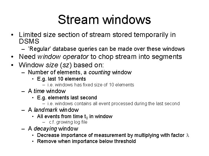
Stream windows • Limited size section of stream stored temporarily in DSMS – ’Regular’ database queries can be made over these windows • Need window operator to chop stream into segments • Window size (sz) based on: – Number of elements, a counting window • E. g. last 10 elements – i. e. windows has fixed size of 10 elements – A time window • E. g. elements last second – i. e. windows contains all event processed during the last second – A landmark window • All events from time t 0 in window – c. f. growing log file – A decaying window • Decrease importance of measurement by multiplying with factor l • Remove when importance below threshold

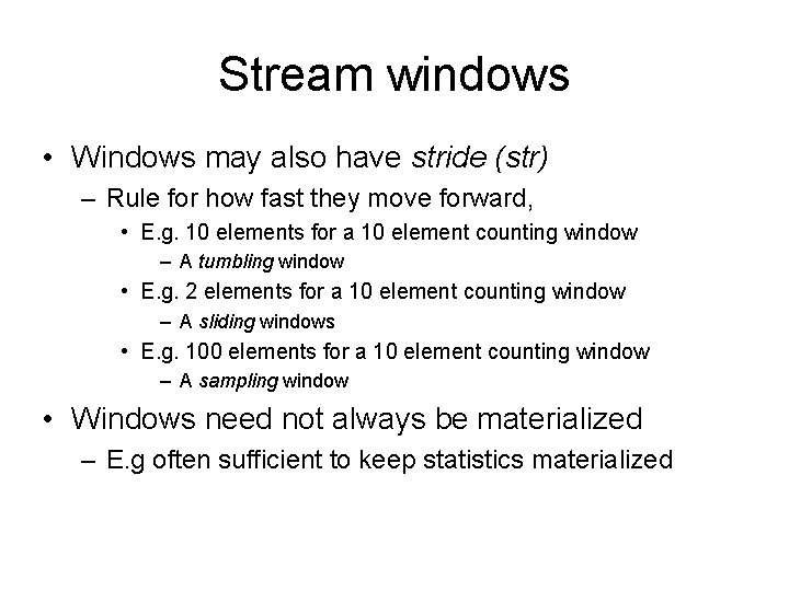
Stream windows • Windows may also have stride (str) – Rule for how fast they move forward, • E. g. 10 elements for a 10 element counting window – A tumbling window • E. g. 2 elements for a 10 element counting window – A sliding windows • E. g. 100 elements for a 10 element counting window – A sampling window • Windows need not always be materialized – E. g often sufficient to keep statistics materialized

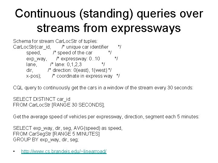
Continuous (standing) queries over streams from expressways Schema for stream Car. Loc. Str of tuples: Car. Loc. Str(car_id, /* unique car identifier */ speed, /* speed of the car */ exp_way, /* expressway: 0. . 10 */ lane, /* lane: 0, 1, 2, 3 */ dir, /* direction: 0(east), 1(west) */ x-pos); /* coordinate in express way */ CQL query to continuously get the cars in a window of the stream every 30 seconds: SELECT DISTINCT car_id FROM Car. Loc. Str [RANGE 30 SECONDS]; Get the average speed of vehicles per expressway, direction, segment each 5 minutes: SELECT exp_way, dir, seg, AVG(speed) as speed, FROM Car. Seg. Str [RANGE 5 MINUTES] GROUP BY exp_way, dir, seg; • http: //www. cs. brandeis. edu/~linearroad/

Denstream • Streamed DBScan • Published: 2006 SIAM Conf. on Data Mining (http: //user. it. uu. se/~torer/Den. Stream. pdf) • Regular DBScan: – DBScan saves cluster memberships of static database per member object in database by scanning database looking for pairs of objects close to each other – Database accessed many times – For scalable processing a spatial index must be used to index points in hyperspace and answer nearest-neighbor queries

Denstream • Denstream – – One pass processing Limited memory Evolving clustering => not static cluster membership Indefinite stream => store cluster memberships not stored in database – No assumption of number of clusters • clusters fade in and fade out – Clusters of arbitrary shape allowed – Good at handling outliers

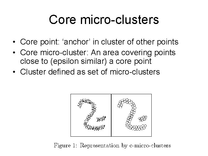
Core micro-clusters • Core point: ‘anchor’ in cluster of other points • Core micro-cluster: An area covering points close to (epsilon similar) a core point • Cluster defined as set of micro-clusters

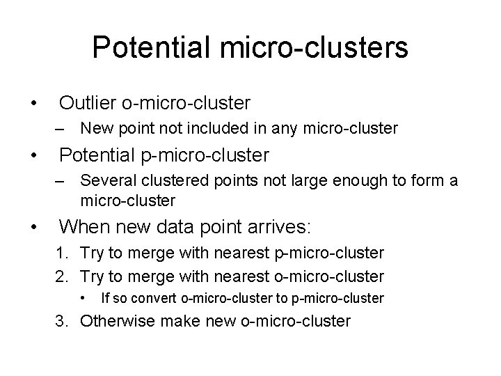
Potential micro-clusters • Outlier o-micro-cluster – New point not included in any micro-cluster • Potential p-micro-cluster – Several clustered points not large enough to form a micro-cluster • When new data point arrives: 1. Try to merge with nearest p-micro-cluster 2. Try to merge with nearest o-micro-cluster • If so convert o-micro-cluster to p-micro-cluster 3. Otherwise make new o-micro-cluster

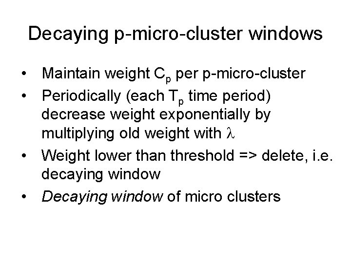
Decaying p-micro-cluster windows • Maintain weight Cp per p-micro-cluster • Periodically (each Tp time period) decrease weight exponentially by multiplying old weight with l • Weight lower than threshold => delete, i. e. decaying window • Decaying window of micro clusters

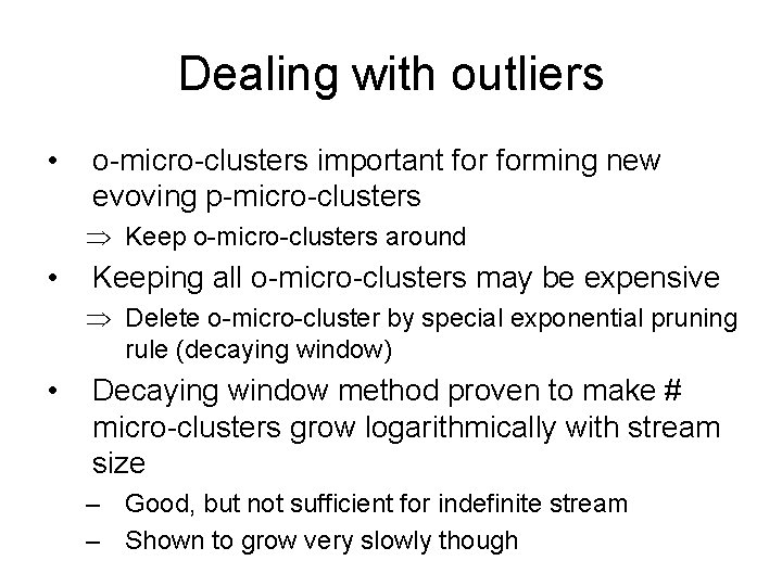
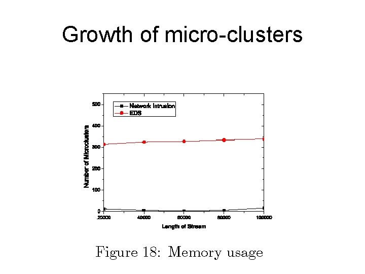
Dealing with outliers • o-micro-clusters important forming new evoving p-micro-clusters Þ Keep o-micro-clusters around • Keeping all o-micro-clusters may be expensive Þ Delete o-micro-cluster by special exponential pruning rule (decaying window) • Decaying window method proven to make # micro-clusters grow logarithmically with stream size – Good, but not sufficient for indefinite stream – Shown to grow very slowly though

Growth of micro-clusters

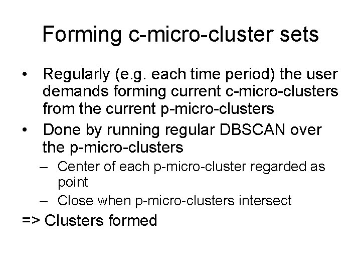
Forming c-micro-cluster sets • Regularly (e. g. each time period) the user demands forming current c-micro-clusters from the current p-micro-clusters • Done by running regular DBSCAN over the p-micro-clusters – Center of each p-micro-cluster regarded as point – Close when p-micro-clusters intersect => Clusters formed

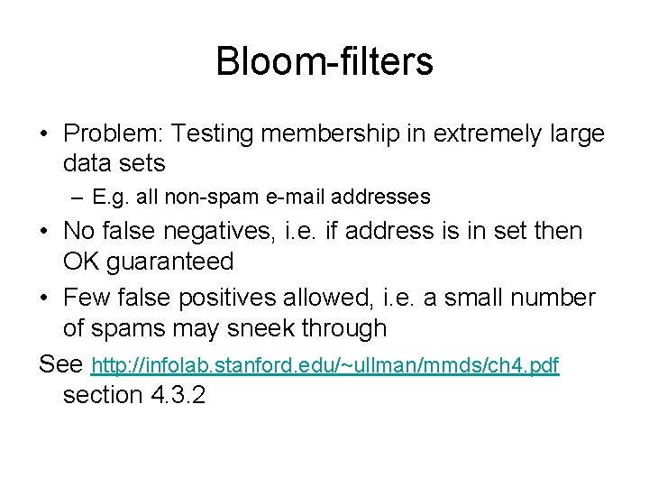
Bloom-filters • Problem: Testing membership in extremely large data sets – E. g. all non-spam e-mail addresses • No false negatives, i. e. if address is in set then OK guaranteed • Few false positives allowed, i. e. a small number of spams may sneek through See http: //infolab. stanford. edu/~ullman/mmds/ch 4. pdf section 4. 3. 2

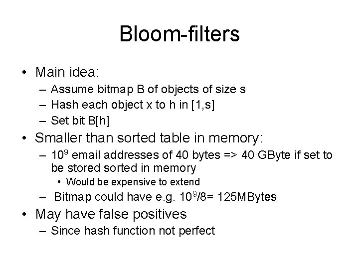
Bloom-filters • Main idea: – Assume bitmap B of objects of size s – Hash each object x to h in [1, s] – Set bit B[h] • Smaller than sorted table in memory: – 109 email addresses of 40 bytes => 40 GByte if set to be stored sorted in memory • Would be expensive to extend – Bitmap could have e. g. 109/8= 125 MBytes • May have false positives – Since hash function not perfect

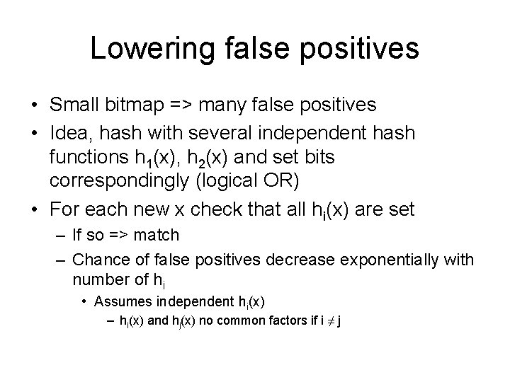
Lowering false positives • Small bitmap => many false positives • Idea, hash with several independent hash functions h 1(x), h 2(x) and set bits correspondingly (logical OR) • For each new x check that all hi(x) are set – If so => match – Chance of false positives decrease exponentially with number of hi • Assumes independent hi(x) – hi(x) and hj(x) no common factors if i ≠ j

Books - Anand Rajaraman & J. Ullman: Mining of Massive Datasets http: //infolab. stanford. edu/~ullman/mmds. html - L. Golab and T. Özsu: Issues in Stream Data Management, SIGMOD Records, 32(2), June 2003, http: //www. acm. org/sigmod/record/issues/ 0306/1. golab-ozsu 1. pdf