Data sets and Visualisation Lesson 5 Prof dr

Data sets and Visualisation Lesson 5 Prof. dr Angelina Njeguš Full Professor at Singidunum University

Agenda ü ü ü File formats Setting the working directory Loading the data Data Visualisation Basic plotting functions

File formats § A file format is a standard way in which information is encoded for storage in a file. ú First, the file format specifies whether the file is a binary or ASCII file. - Ascii mode transfers files as ‘text’. Examples of ASCII files would be. txt, . asp, . html, and. php files - Binary mode transfers files as raw data. Examples of binary files would be. wav, . jpg, . gif, and mp 3 files ú Second, it shows how the information is organized. For example, comma-separated values (CSV) file format stores tabular data in plain text.

The most used file formats § CSV file (Comma-Separated Values, CSV): ú plain text file which contains a list of data. ú these files are often used for the exchange of data between different applications. ú they often use the comma character to separate data, but sometimes use other characters such as semicolons § Binary file: ú a file which contains information present only in the form of bits and bytes (0's and 1's). ú they are not human-readable because the bytes translate into characters and symbols that contain many other non-printable characters. If we will read a binary file using any text editor, it will show the characters like ð and Ø. § JSON file (Java. Script Object Notation): ú an open standard file format, and data interchange format, that uses human-readable text to store and transmit data objects consisting of attribute–value pairs and array data types (or any other serializable value).

Which file formats can be read by R? § A very important feature of all programming languages is the ability to communicate with the outside world, i. e. import and export data, whch includes: ú ú reading and writing simple text files from your local hard disc, download and reading data from the web (e. g. , JSON, xml, html), read and write more complex files like Net. CDF or geotiff, xlsx files, select and insert data into data bases, etc. § Base R comes with “basic” functionality to handle some common file types, for more advanced or specialized file formats (or connections) additional packages need to be installed. Some R packages are: ú ú ú rjson to read/parse JSON data, xml 2 to read, parse, manipulate, create, and save xml files, png and jpeg to read png/jpg images, ncdf 4 to read net. CDF files, RSQLite to read and write SQLite files, RMy. SQL to connect to My. SQL data bases.

Loading in the Data § Datasets can either be built-in or can be loaded from external sources in R. ú Built-in datasets refer to the datasets already provided within R. - To see the list of pre-loaded data, type the function data(). To load the built-in dataset into the R type: data(airquality). For more info about built-in dataset type: ? airquality To see all data, just type: airquality To see just first 10 rows of the dataset: head(airquality, 10) To view as a data frame type: View(airquality) (Note: View() is with capital letter V) ú In case of an External data source (CSV, Excel, text, HTML file etc. ), simply set the folder containing the data as the working directory with the setwd() command. path <- 'https: //raw. githubusercontent. com/guru 99 -edu/R-Programming/master/titanic_data. csv' titanic <-read. csv(path) head(titanic)

Getting and setting the working directory • R allows us to read data from files which • Example are stored outside the R environment. • The file can be present in the current working directory so that R can read it, but we can also set our directory and read file from there. • The getwd() function is used to check on which directory the R workspace is pointing. • The setwd() function is used to set a new working directory to read and write files from that directory. # Getting and printing current working directory. print(getwd()) [1] "C: /Users/korisnik/Documents" # Setting the current working directory. setwd("C: /Users/korisnik") # setwd("/web/com") # Getting and printing the current working directory. print(getwd()) [1] "C: /Users/korisnik"

Load Data in R Studio • The easiest way to load data into memory in R is by using the R Studio menu items. • R Studio has menu items for loading data in two different places. • The first is in the toolbar of the upper right section of R Studio. • The second is from the top menu of R Studio, go to File > Import Dataset >…

Load the data from § Go to https: //www. kaggle. com/kaggle/sf-salaries. § Download Salaries. csv dataset (15. 5 MB) § Import Salaries. csv into R. § Analyse data: ú What is the structure of the dataset? str(Salaries. csv) ú Get the maximum Total. Pay salary from data frame: max_sal<- max(Salaries$Total. Pay) ú Get the detais of the person who have maximum salary: details <- subset(Salaries, Total. Pay==max(Total. Pay)) ú Get the details of all those whose status is part time (PT) : PTEmpl=subset(Salaries, Status=="PT")

Data Visualisation § With ever increasing volume of data, it is impossible to tell stories without visualisations. § Data visualisation is an art of how to turn numbers into useful knowledge.

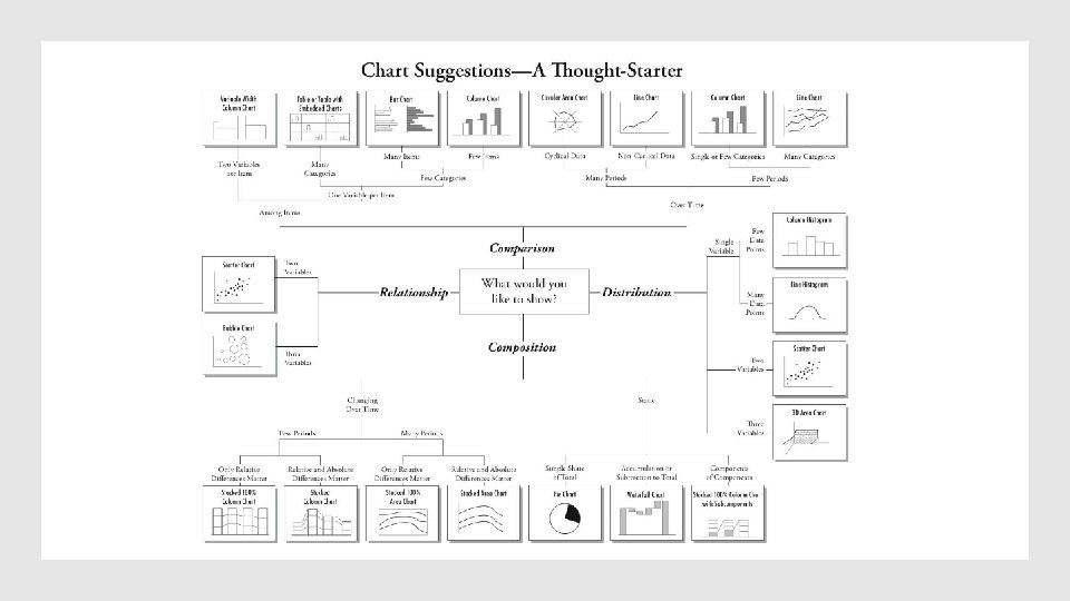
Selecting the Right Chart Type § There are four basic presentation types: ú ú Relationship Distribution Composition Comparison § See the figure on the next slide >>

Chart types 1. 2. 3. 4. 5. 6. 7. Scatter Plot Histogram Bar & Stack Bar Chart Box Plot Area Chart Heat Map Correlogram To get familiar with graphics in R type: demo(graphics), and demo(persp).

1. Scatter Plot § When to use: Scatter Plot is used to see the relationship between two continuous variables. ú For example, if we want to visualise the correlation between items price per their cost data. § Try: data(mtcars) # Import mtcars pairs(~wt+mpg+disp+cyl, data = mtcars, main = "Scatterplot Matrix")

How to read scatter plot • Red box is a scatter plot of x=wt, y=mpg • Sky Blue box is a scatter plot of x=wt, y=disp • Purple box is a scatter plot of x=wt, y=cyl • Pink box is a scatter plot of x=disp, y=cyl (see the pattern? ) • Orange box is a scatter plot of x=mpg, y=wt (red box with switched axis)

How to interpret the content of the scatter plot § Scatter plots help us understand the association (correlaton, relationship) between two variables using: ú ú Direction: Positive or Negative Form: Linear or Non linear Strength: Weak, Moderate or Strong Outliers

What is correlation?

Why direction is important? Positive dependency Negative dependancy Variables depend on each other two variables do not depend on each other

Form of the curve • Linear • Non linear • E. g. strong – non linear means that there is a pattern, but the form is non linear.

Strength of the curve strong moderate perfect weak no association

Outliners Outliner Probably you will want to remove outliners, to see patterns.

What is the difference between correlation and regression?

Intro to plot() function § The most used plotting function in R programming is the plot() function. ú It is a generic function, meaning, it has many methods which are called according to the type of object passed to plot(). ú In the simplest case, we can pass in a vector and we will get a scatter plot of magnitude vs index. But generally, we pass in two vectors and a scatter plot of these points are plotted. § For example, the command plot(c(1, 2), c(3, 5)) would plot the points (1, 3) and (2, 5).

Let’s plot # import mtcars dataset using data("mtcars") x <- mtcars$wt y <- mtcars$hp # Plot with main and axis titles # Change point shape (pch = 15) and remove frame. plot(x, y, main = "Relationship between weight of the car, and Gross horsepower", xlab = "Weight (1000 lbs)", ylab = "Gross horsepower", pch = 15, frame = FALSE) # Add regression line abline(lm(y ~ x, data = mtcars), col = "blue")

Basic plotting functions § There are three basic plotting functions in R: ú high-level plots - creates a complete plot ú low-level plots - adds to an existing plot ú layout command par

High-Level Plot Functions § Some of the basic plot functions include: § Read States 03 dataset and use barplot to show the regions, and histogram to show poverty percentage: States 03 <- read. csv("http: //sites. google. com/site/chiharahesterberg/States 03. csv") barplot(table(States 03$Region)) hist(States 03$Poverty)

Two approaches of creating a scatter plot 1. Provide the plot command with the x-variable, then the y-variable: plot(States 03$Unemp, States 03$Poverty, xlab = "Unemployment", ylab = "Poverty") 2. If the data are contained in a data frame, then provide the names of the variable Y ∼ X along with the name of the data frame. plot(Poverty ~ Unemp, data = States 03, xlab = "Unemployment", ylab = "Poverty")

Optional arguments § High-level functions may also take optional arguments that enhance the plot: Try: hist(States 03$Poverty, main = "Poverty", xlab = "percent", xlim = c(0, 24), ylim = c(0, 20))

Try optional arguments plot(1: 19, pch = 1: 19, xlab = "x", ylab = "y")

Try optional arguments § To plot smooth curves, use the curve command. The first argument must be an expression in terms of x: curve(x^2, from = 0, to = 2) curve(cos(x), from = 0, to = pi, lty = 4, col = "red")

Low-level Plot Functions § Low-level plot functions can be executed only after a high-level plot has been created.

Try low-level plot functions plot(Poverty ~ Unemp, data = States 03, xlab = "Unemployment", ylab = "Poverty") abline(v = mean(States 03$Unemp), lty = 2) #vertical line at mean unemployment rate text(30, 18, "mean unemployment rate") #text at (30, 18) title("Data from 2003") The abline function has several options: • • • abline(3, 5) adds the straight line y = 3 + 5 x abline(v = 2) adds the vertical line, x = 2 abline(h = 0) adds the horizontal line, y = 0

Add a legend points(Uninsured ~ Col. Grad, data = States 03, col = "red", pch = 19) mtext("Percent uninsured", side = 4) legend("bottomleft", legend = c("Y: Poverty", "Y: Uninsured"), col = c("blue", "red"), pch = c(16, 16))

Different plotting symbols for different levels § You can also use different plotting symbols for different levels of a factor variable: range(States 03$Poverty) range(States 03$Col. Grad) plot(Poverty ~ Col. Grad, data = States 03, pch=16, subset=Region=="West", xlim = c(15, 40), ylim = c(5, 20)) points(Poverty ~ Col. Grad, data = States 03, pch=16, col = "red", subset = Region=="South") points(Poverty ~ Col. Grad, data = States 03, pch=16, col = "green", subset = Region=="Northeast") points(Poverty ~ Col. Grad, data = States 03, pch = 16, col = "blue", subset = Region=="Midwest") legend("topright", legend=c("West", "South", "Northeast", "Midwest"), pch = rep(16, 4), col = c("black", "red", "green", "blue"))

How to show curves? curve(cos(x), from = 0, to = 2*pi) curve(sin(x), add = TRUE, col = "blue", lty = 2)

The par Command § In addition to low-level plotting commands, the presentation of graphics can be improved with graphical parameters. § They can be used either as options of graphic functions (but it does not work for all), or with the function par to change permanently the graphical parameters, i. e. the subsequent plots will be drawn with respect to the parameters specified by the user. § For instance, type the following command: par(bg="yellow") #Import States 03 dataset hist(States 03$Teachers. Pay, main = "Teachers Pay", xlab = "percent") This will result that all subsequent plots will be drawn with a yellow background. To see all colors, type: colors() Type dev. off() to close graphics device

Exercise: with par command show multifigure by row § Try the option mfrow for multi-figure, by row, or mfcol, by column. ú This will result, that all subsequent plots will be shown together. ú To change it back to the default, type mfrow=c(1, 1). § For example, to have a 3 x 2 layout where the plots are added by row, set: par(mfrow = c(2, 3)) #2 x 3 layout by row hist(States 03$Poverty, main = "Poverty", xlab = "percent") #repeat this line 6 times

R Graphic Packages • R has 3 main packages for data visualisation: • Graphics – It is part of R installation and is the fundamental package for visualizing data. All the basic plots can be created using this package. • dgplot 2 – it has structured approach to data visualisation and builds upon the features available in Graphics and Lattice packages. • Lattice – it is a powerful data visualisation system with an emphasis on multivariate data (simultaneous study of several variables).

Some more R Visualisation Packages • plotly - The plotly package provides online interactive and quality graphs. This package extends upon the Java. Script library ? plotly. js. • tidyquant - The tidyquant is a financial package that is used for carrying out quantitative financial analysis. This package adds under tidyverse universe as a financial package that is used for importing, analyzing, and visualizing the data. • taucharts - The library provides a declarative interface for rapid mapping of data fields to visual properties. • ggiraph - It is a tool that allows us to create dynamic ggplot graphs. This package allows us to add tooltips, Java. Script actions, and animations to the graphics. • geofacets - This package provides geofaceting functionality for 'ggplot 2'. Geofaceting arranges a sequence of plots for different geographical entities into a grid that preserves some of the geographical orientation.

Overview of the high-level graphical functions in R

Overview of the low-level plotting commands

Overview of par commands § Type ? par to list all par commands

Useful links § Plots in R: https: //af 911380 -a-62 cb 3 a 1 a-s-sites. googlegroups. com/site/chiharahesterberg/rtutorials/RPlot. pdf? attachauth=ANo. Y 7 crd. JNf. XMov. Gu. FJBLYL 77 y 6 h. Qz 2_C 93 QQk. Kmsa-9 s. Rkm-J 3 -K- ez. Iy 35 q. An. LHya. Cy. Eb_sm. QZZTo 81 NIOYOdl 8 HZw 7 s. Vu. C 3 e 7 BTELG 376 ogd-bk. EWTWs. Z 2 Zc. Rj. Y 5 p 1 mh 4 rz. KXSNTP 0 ETe. We. OL 7 s. Wx. Bmt 19 z. Wu 93 ac 1 b. D 6 p. U 1 HYe. Aa. HUl. Htq__wc. AV 0 Ec. TRp. AXUw. ITWh 8 dd. IUbtmlfs. R 55 -4 v. FFy. JCf. Bu 7 lpk. AJjui 7 e. IYup. Del 5 E%3 D&attredirects=1 § R for Beginners by Emmanuel Paradis: https: //cran. r-project. org/doc/contrib/Paradis-rdebuts_en. pdf