Data Science Classification Decision Trees Lecture Notes for

Data Science Classification: Decision Trees Lecture Notes for Chapter 4 Tan, Steinbach, Kumar © Tan, Steinbach, Kumar Introduction to Data Mining 4/18/2004 1

Overview l l Classification is one core task of data mining. There are two chapters to introduce classification in our textbook： – Chapter 4 introduces the basic concepts of classification and one classification algorithm Decision tree, as well as some key issues such as model overfitting and model evaluation. – Chapter 5 introduces some other commonly used classification algorithms such as Bayesian Classifiers, artificial neural network and ensemble classifiers. © Tan, Steinbach, Kumar

Classification: Definition l Classification is a pervasive problem and it has a broad of applications. – detect spam email messages based on the message header and content – categorize cells as malignant or benign based on the results of MRI scans – classify galaxies based on their shapes l So, what is the definition of classification? © Tan, Steinbach, Kumar

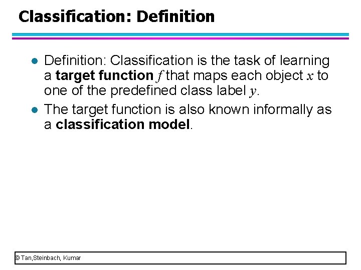
Classification: Definition l l Definition: Classification is the task of learning a target function f that maps each object x to one of the predefined class label y. The target function is also known informally as a classification model. © Tan, Steinbach, Kumar

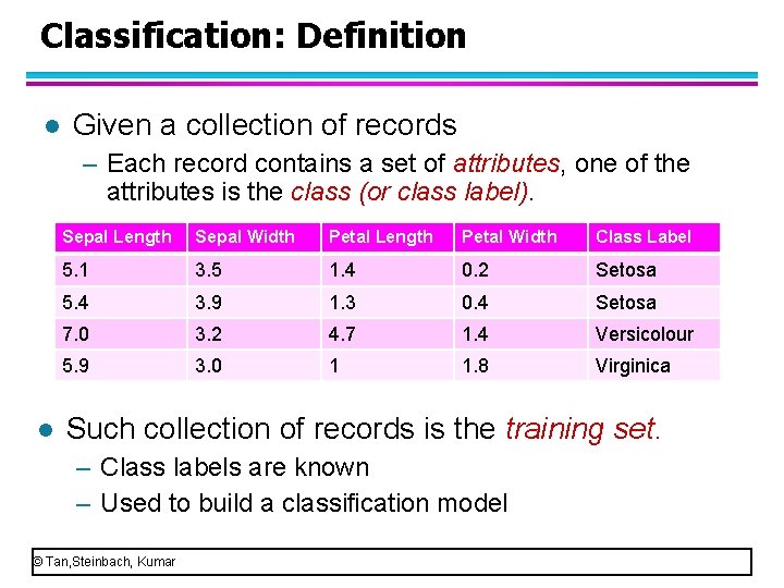
Classification: Definition l Given a collection of records – Each record contains a set of attributes, one of the attributes is the class (or class label). l Sepal Length Sepal Width Petal Length Petal Width Class Label 5. 1 3. 5 1. 4 0. 2 Setosa 5. 4 3. 9 1. 3 0. 4 Setosa 7. 0 3. 2 4. 7 1. 4 Versicolour 5. 9 3. 0 1 1. 8 Virginica Such collection of records is the training set. – Class labels are known – Used to build a classification model © Tan, Steinbach, Kumar

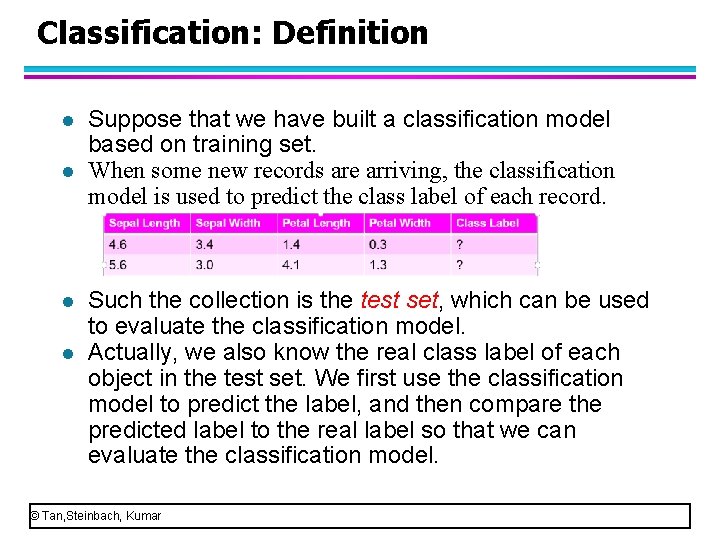
Classification: Definition l l Suppose that we have built a classification model based on training set. When some new records are arriving, the classification model is used to predict the class label of each record. Such the collection is the test set, which can be used to evaluate the classification model. Actually, we also know the real class label of each object in the test set. We first use the classification model to predict the label, and then compare the predicted label to the real label so that we can evaluate the classification model. © Tan, Steinbach, Kumar

Classification: Definition l l Generally, to evaluate a classification model, we divide the given data set (the class label of each object is known) into training set and test set. The training set is used to build the model and the test set is used to evaluate the model. Once a classification model is built and validated, it can be used to predict the class label of unknown records. We will learn to evaluate a classification model in detail latter. © Tan, Steinbach, Kumar

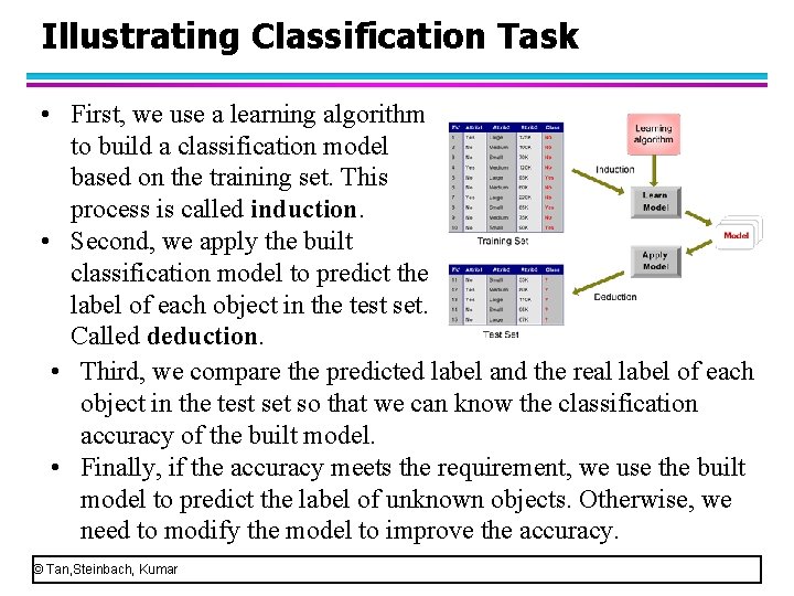
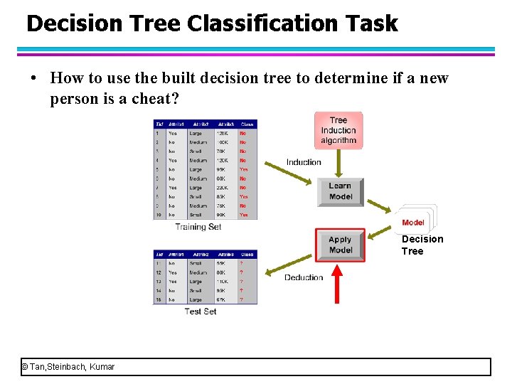
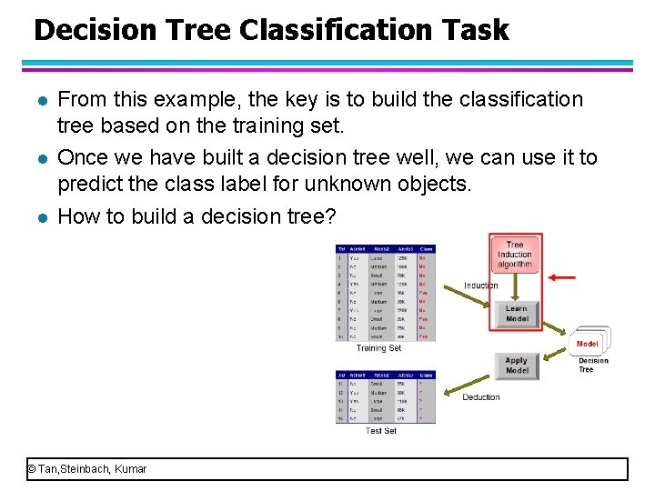
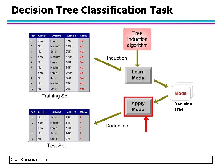
Illustrating Classification Task • First, we use a learning algorithm to build a classification model based on the training set. This process is called induction. • Second, we apply the built classification model to predict the label of each object in the test set. Called deduction. • Third, we compare the predicted label and the real label of each object in the test set so that we can know the classification accuracy of the built model. • Finally, if the accuracy meets the requirement, we use the built model to predict the label of unknown objects. Otherwise, we need to modify the model to improve the accuracy. © Tan, Steinbach, Kumar

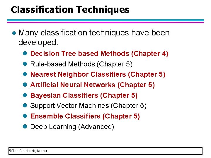
Classification Techniques l Many classification techniques have been developed: l l l l Decision Tree based Methods (Chapter 4) Rule-based Methods (Chapter 5) Nearest Neighbor Classifiers (Chapter 5) Artificial Neural Networks (Chapter 5) Bayesian Classifiers (Chapter 5) Support Vector Machines (Chapter 5) Ensemble Classifiers (Chapter 5) Deep Learning (Advanced) © Tan, Steinbach, Kumar

Classification Concepts l. Section 1: Decision Tree © Tan, Steinbach, Kumar

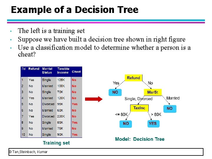
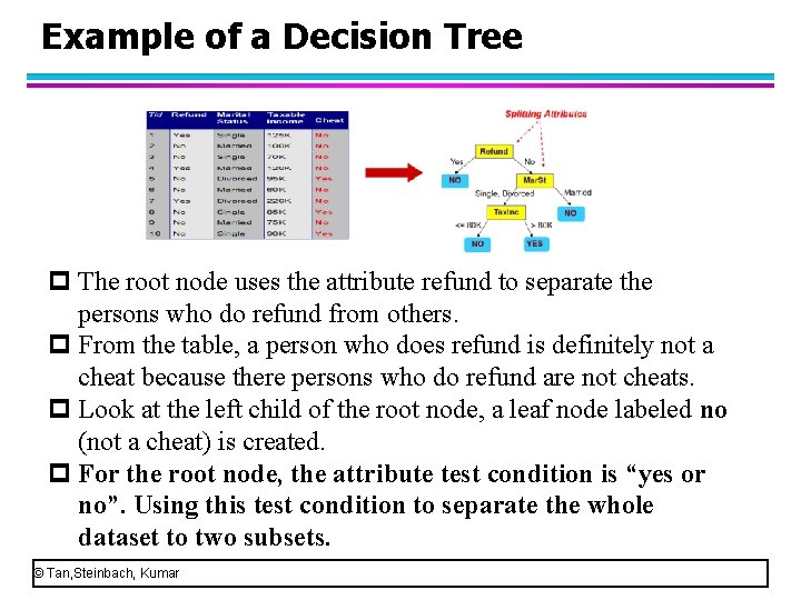
Example of a Decision Tree • • • The left is a training set Suppose we have built a decision tree shown in right figure Use a classification model to determine whether a person is a cheat? © Tan, Steinbach, Kumar

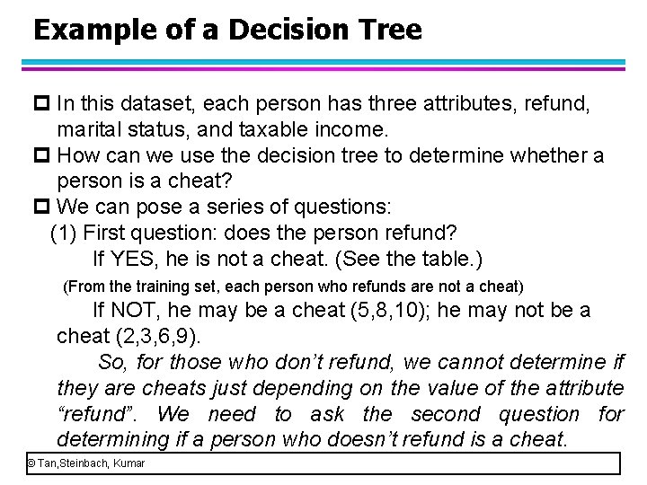
Example of a Decision Tree p In this dataset, each person has three attributes, refund, marital status, and taxable income. p How can we use the decision tree to determine whether a person is a cheat? p We can pose a series of questions: (1) First question: does the person refund? If YES, he is not a cheat. (See the table. ) (From the training set, each person who refunds are not a cheat) If NOT, he may be a cheat (5, 8, 10); he may not be a cheat (2, 3, 6, 9). So, for those who don’t refund, we cannot determine if they are cheats just depending on the value of the attribute “refund”. We need to ask the second question for determining if a person who doesn’t refund is a cheat. © Tan, Steinbach, Kumar

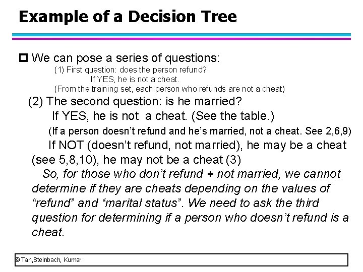
Example of a Decision Tree p We can pose a series of questions: (1) First question: does the person refund? If YES, he is not a cheat. (From the training set, each person who refunds are not a cheat) (2) The second question: is he married? If YES, he is not a cheat. (See the table. ) (If a person doesn’t refund and he’s married, not a cheat. See 2, 6, 9) If NOT (doesn’t refund, not married), he may be a cheat (see 5, 8, 10), he may not be a cheat (3) So, for those who don’t refund + not married, we cannot determine if they are cheats depending on the values of “refund” and “marital status”. We need to ask the third question for determining if a person who doesn’t refund is a cheat. © Tan, Steinbach, Kumar

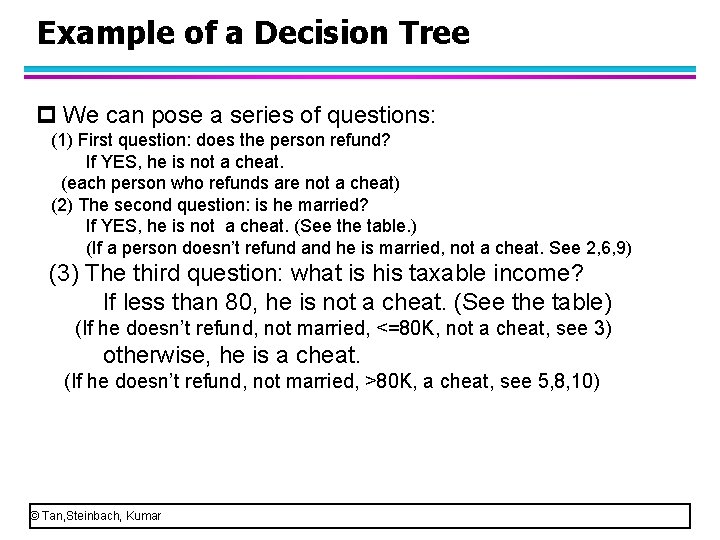
Example of a Decision Tree p We can pose a series of questions: (1) First question: does the person refund? If YES, he is not a cheat. (each person who refunds are not a cheat) (2) The second question: is he married? If YES, he is not a cheat. (See the table. ) (If a person doesn’t refund and he is married, not a cheat. See 2, 6, 9) (3) The third question: what is his taxable income? If less than 80, he is not a cheat. (See the table) (If he doesn’t refund, not married, <=80 K, not a cheat, see 3) otherwise, he is a cheat. (If he doesn’t refund, not married, >80 K, a cheat, see 5, 8, 10) © Tan, Steinbach, Kumar

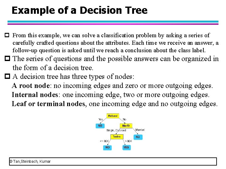
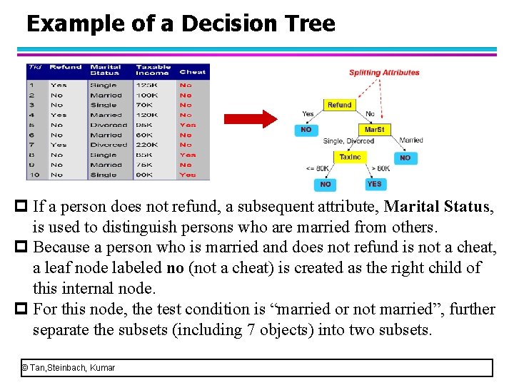
Example of a Decision Tree p From this example, we can solve a classification problem by asking a series of carefully crafted questions about the attributes. Each time we receive an answer, a follow-up question is asked until we reach a conclusion about the class label. p The series of questions and the possible answers can be organized in the form of a decision tree. p A decision tree has three types of nodes: A root node: no incoming edges and zero or more outgoing edges. Internal nodes: one incoming edge, two or more outgoing edges. Leaf or terminal nodes, one incoming edge and no outgoing edges. © Tan, Steinbach, Kumar

Example of a Decision Tree p A decision tree has three types of nodes: A root node, Internal nodes, Leaf or terminal nodes. p Each leaf node is assigned to a class label. p The non-terminal nodes (root node and internal nodes) contain attribute test conditions to separate records that have different characteristics. © Tan, Steinbach, Kumar

Example of a Decision Tree p The root node uses the attribute refund to separate the persons who do refund from others. p From the table, a person who does refund is definitely not a cheat because there persons who do refund are not cheats. p Look at the left child of the root node, a leaf node labeled no (not a cheat) is created. p For the root node, the attribute test condition is “yes or no”. Using this test condition to separate the whole dataset to two subsets. © Tan, Steinbach, Kumar

Example of a Decision Tree p If a person does not refund, a subsequent attribute, Marital Status, is used to distinguish persons who are married from others. p Because a person who is married and does not refund is not a cheat, a leaf node labeled no (not a cheat) is created as the right child of this internal node. p For this node, the test condition is “married or not married”, further separate the subsets (including 7 objects) into two subsets. © Tan, Steinbach, Kumar

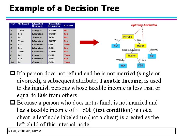
Example of a Decision Tree p If a person does not refund and he is not married (single or divorced), a subsequent attribute, Taxable Income, is used to distinguish persons whose taxable income is less than or equal to 80 k from others. p Because a person who does not refund, is not married and has a taxable income of <=80 k (test condition) is not a cheat, a leaf node labeled no (not a cheat) is created as the left child of this internal node. © Tan, Steinbach, Kumar

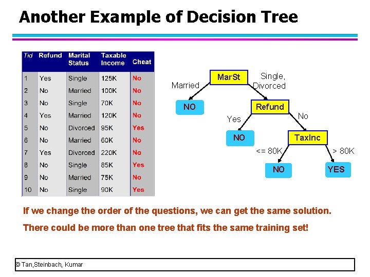
Another Example of Decision Tree Married Mar. St NO Single, Divorced Refund No Yes NO Tax. Inc <= 80 K NO > 80 K YES If we change the order of the questions, we can get the same solution. There could be more than one tree that fits the same training set! © Tan, Steinbach, Kumar

Decision Tree Classification Task • How to use the built decision tree to determine if a new person is a cheat? Decision Tree © Tan, Steinbach, Kumar

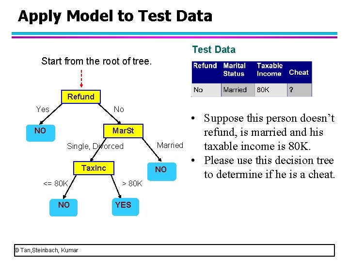
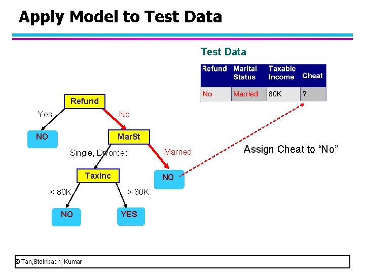
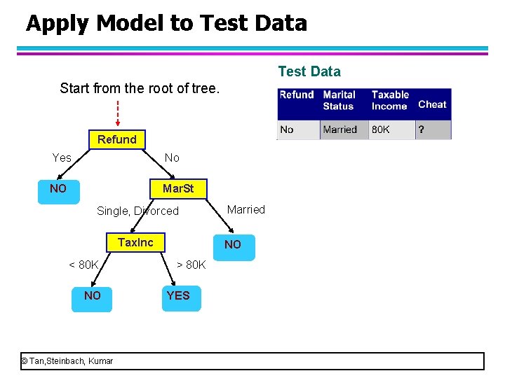
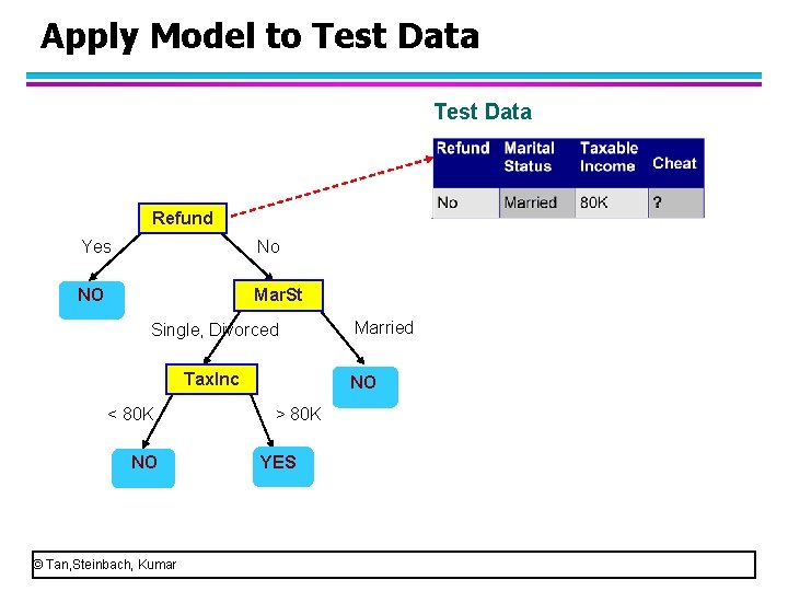
Apply Model to Test Data Start from the root of tree. Refund Yes No NO Mar. St Single, Divorced Tax. Inc <= 80 K NO © Tan, Steinbach, Kumar Married NO > 80 K YES • Suppose this person doesn’t refund, is married and his taxable income is 80 K. • Please use this decision tree to determine if he is a cheat.

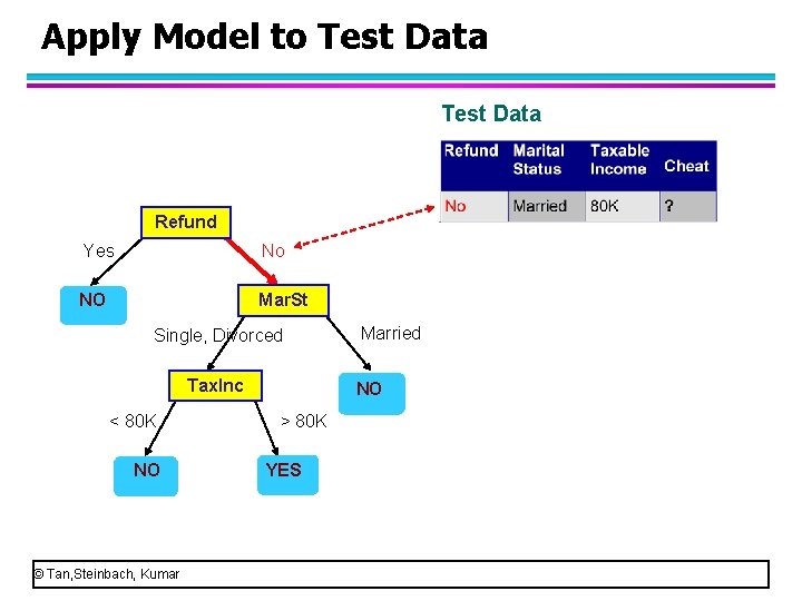
Apply Model to Test Data Refund Yes No NO Mar. St Single, Divorced Tax. Inc < 80 K NO © Tan, Steinbach, Kumar Married NO > 80 K YES • Start from the root node. • Look at the value of refund. • Since the value of refund is “no”, we go to the right child tree.

Apply Model to Test Data Refund Yes No NO Mar. St Single, Divorced Tax. Inc < 80 K NO © Tan, Steinbach, Kumar Married NO > 80 K YES

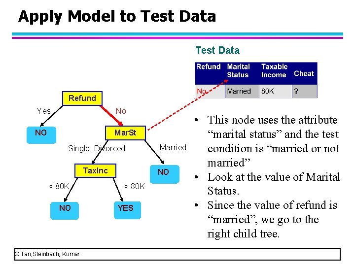
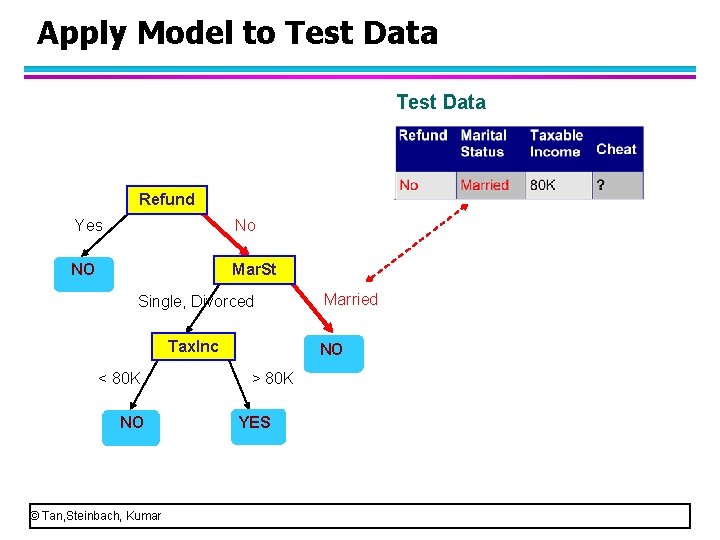
Apply Model to Test Data Refund Yes No NO Mar. St Single, Divorced Tax. Inc < 80 K NO © Tan, Steinbach, Kumar Married NO > 80 K YES • This node uses the attribute “marital status” and the test condition is “married or not married” • Look at the value of Marital Status. • Since the value of refund is “married”, we go to the right child tree.

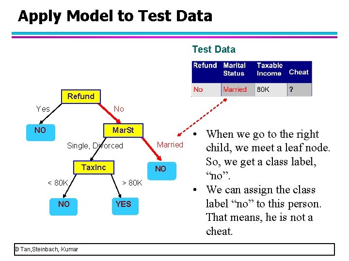
Apply Model to Test Data Refund Yes No NO Mar. St Single, Divorced Tax. Inc < 80 K NO © Tan, Steinbach, Kumar Married NO > 80 K YES • When we go to the right child, we meet a leaf node. So, we get a class label, “no”. • We can assign the class label “no” to this person. That means, he is not a cheat.

Apply Model to Test Data Refund Yes No NO Mar. St Single, Divorced Tax. Inc < 80 K NO © Tan, Steinbach, Kumar Married NO > 80 K YES Assign Cheat to “No”

Decision Tree Classification Task l l l From this example, the key is to build the classification tree based on the training set. Once we have built a decision tree well, we can use it to predict the class label for unknown objects. How to build a decision tree? © Tan, Steinbach, Kumar

Decision Tree Induction Many Algorithms have been presented: – Hunt’s Algorithm – CART – ID 3, C 4. 5 – SLIQ, SPRINT l Hunt’s algorithm is the basic method for building a decision tree. We focus on this algorithm in this course. l Once you understand Hunt’s algorithm, you can easily learn other algorithms. l © Tan, Steinbach, Kumar

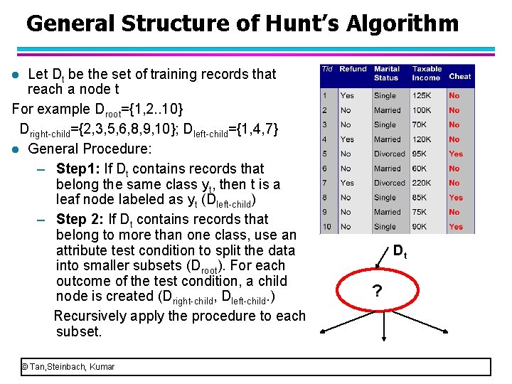
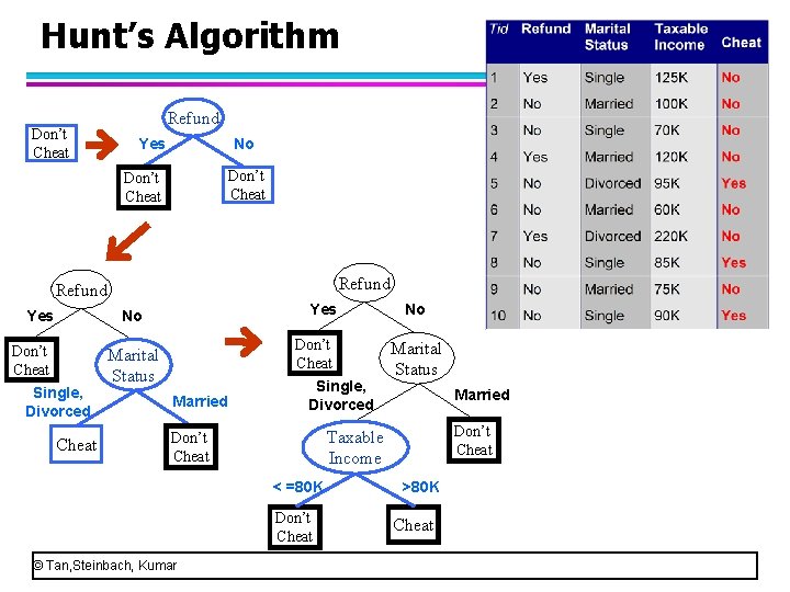
General Structure of Hunt’s Algorithm Let Dt be the set of training records that reach a node t For example Droot={1, 2. . 10} Dright-child={2, 3, 5, 6, 8, 9, 10}; Dleft-child={1, 4, 7} l General Procedure: – Step 1: If Dt contains records that belong the same class yt, then t is a leaf node labeled as yt (Dleft-child) – Step 2: If Dt contains records that belong to more than one class, use an attribute test condition to split the data into smaller subsets (Droot). For each outcome of the test condition, a child node is created (Dright-child, Dleft-child. ) Recursively apply the procedure to each subset. l © Tan, Steinbach, Kumar Dt ?

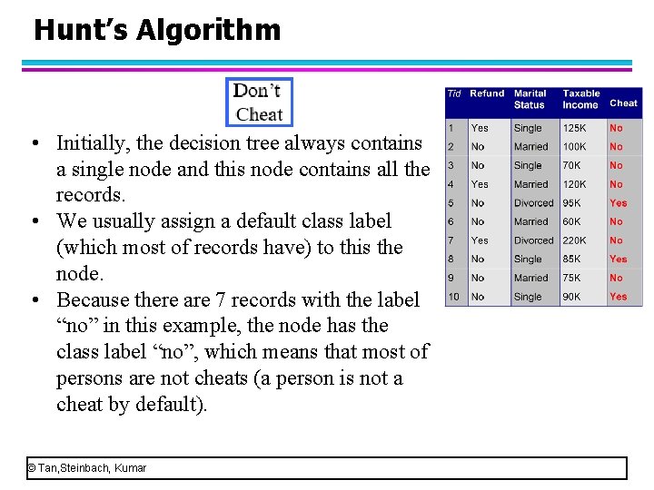
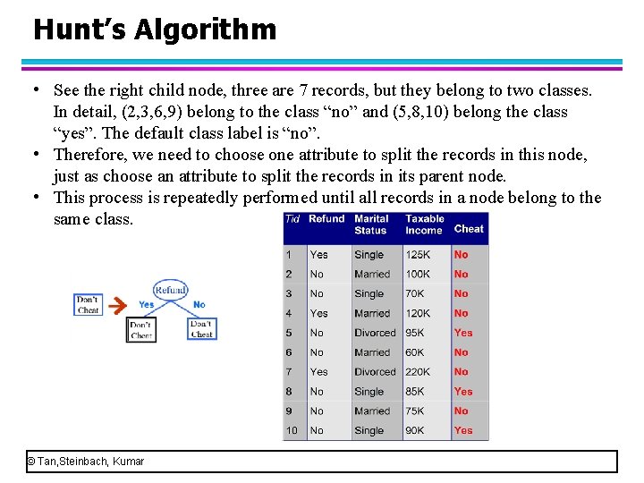
Hunt’s Algorithm • Initially, the decision tree always contains a single node and this node contains all the records. • We usually assign a default class label (which most of records have) to this the node. • Because there are 7 records with the label “no” in this example, the node has the class label “no”, which means that most of persons are not cheats (a person is not a cheat by default). © Tan, Steinbach, Kumar

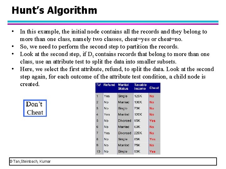
Hunt’s Algorithm • In this example, the initial node contains all the records and they belong to more than one class, namely two classes, cheat=yes or cheat=no. • So, we need to perform the second step to partition the records. • Look at the second step, if Dt contains records that belong to more than one class, use an attribute test to split the data into smaller subsets. • Here, we select the first attribute, refund, to split the data. Look at the second step again, for each outcome of the attribute test condition, a child node is created. © Tan, Steinbach, Kumar

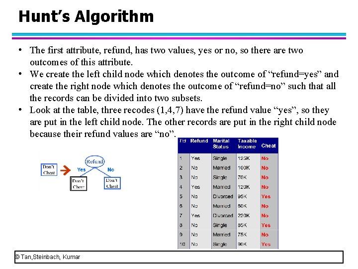
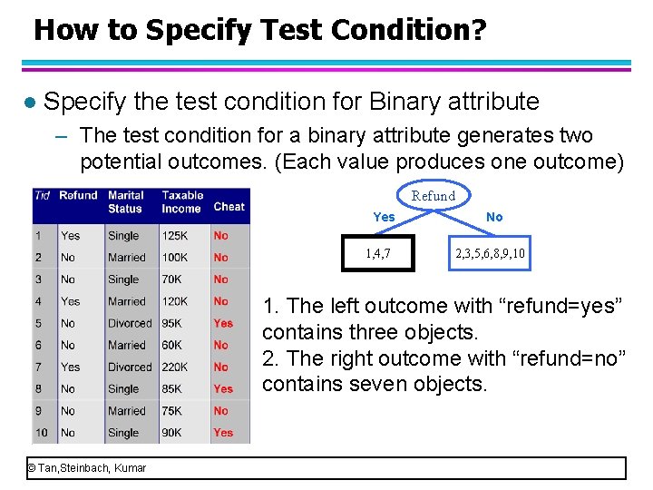
Hunt’s Algorithm • The first attribute, refund, has two values, yes or no, so there are two outcomes of this attribute. • We create the left child node which denotes the outcome of “refund=yes” and create the right node which denotes the outcome of “refund=no” such that all the records can be divided into two subsets. • Look at the table, three recodes (1, 4, 7) have the refund value “yes”, so they are put in the left child node. The other records are put in the right child node because their refund values are “no”. © Tan, Steinbach, Kumar

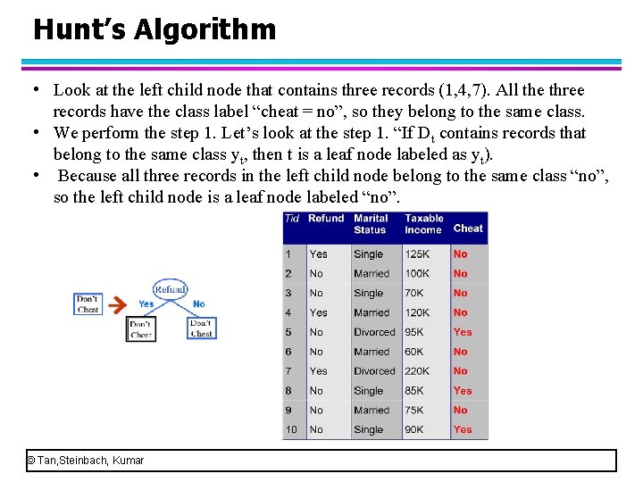
Hunt’s Algorithm • Look at the left child node that contains three records (1, 4, 7). All the three records have the class label “cheat = no”, so they belong to the same class. • We perform the step 1. Let’s look at the step 1. “If Dt contains records that belong to the same class yt, then t is a leaf node labeled as yt). • Because all three records in the left child node belong to the same class “no”, so the left child node is a leaf node labeled “no”. © Tan, Steinbach, Kumar

Hunt’s Algorithm • See the right child node, three are 7 records, but they belong to two classes. In detail, (2, 3, 6, 9) belong to the class “no” and (5, 8, 10) belong the class “yes”. The default class label is “no”. • Therefore, we need to choose one attribute to split the records in this node, just as choose an attribute to split the records in its parent node. • This process is repeatedly performed until all records in a node belong to the same class. © Tan, Steinbach, Kumar

Hunt’s Algorithm Don’t Cheat Refund Yes No Don’t Cheat Single, Divorced Cheat Don’t Cheat Marital Status Married Single, Divorced Marital Status Married Don’t Cheat Taxable Income Don’t Cheat < =80 K Don’t Cheat © Tan, Steinbach, Kumar No >80 K Cheat

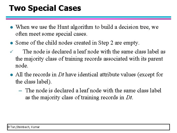
Two Special Cases l l ü l When we use the Hunt algorithm to build a decision tree, we often meet some special cases. Some of the child nodes created in Step 2 are empty. The node is declared a leaf node with the same class label as the majority class of training records associated with its parent node. All the records in Dt have identical attribute values (except for the class label). – The node is declared a leaf node with the same class label as the majority class of training records in Dt. © Tan, Steinbach, Kumar

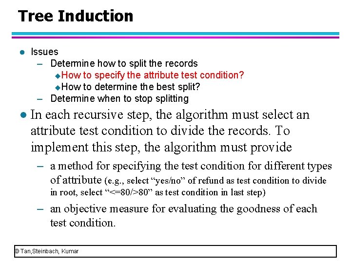
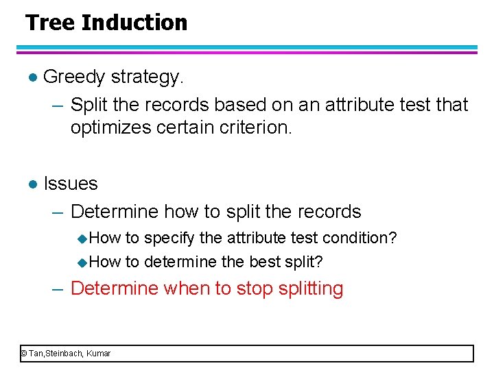
Tree Induction l Decision tree-based algorithm is a Greedy strategy. – Split the records based on an attribute test condition that optimizes certain criterion. l When we use the Hunt Algorithm two issues must be addressed – Determine how to split the records u. How to specify the attribute test condition? u. How to determine the best split? – Determine when to stop splitting © Tan, Steinbach, Kumar

Tree Induction l Issues – Determine how to split the records u. How to specify the attribute test condition? u. How to determine the best split? – Determine when to stop splitting l In each recursive step, the algorithm must select an attribute test condition to divide the records. To implement this step, the algorithm must provide – a method for specifying the test condition for different types of attribute (e. g. , select “yes/no” of refund as test condition to divide in root, select “<=80/>80” as test condition in last step) – an objective measure for evaluating the goodness of each test condition. © Tan, Steinbach, Kumar

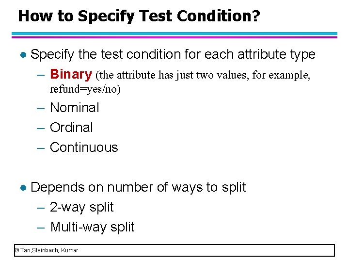
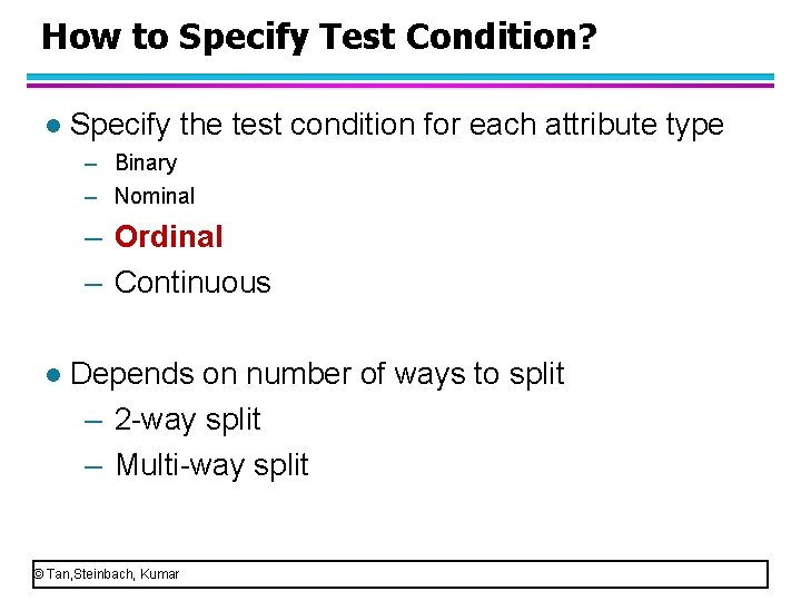
How to Specify Test Condition? l Specify the test condition for each attribute type – Binary (the attribute has just two values, for example, refund=yes/no) – Nominal – Ordinal – Continuous l Depends on number of ways to split – 2 -way split – Multi-way split © Tan, Steinbach, Kumar

How to Specify Test Condition? l Specify the test condition for Binary attribute – The test condition for a binary attribute generates two potential outcomes. (Each value produces one outcome) Refund Yes 1, 4, 7 No 2, 3, 5, 6, 8, 9, 10 1. The left outcome with “refund=yes” contains three objects. 2. The right outcome with “refund=no” contains seven objects. © Tan, Steinbach, Kumar

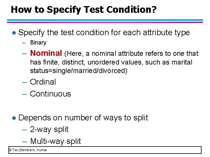
How to Specify Test Condition? l Specify the test condition for each attribute type – Binary – Nominal (Here, a nominal attribute refers to one that has finite, distinct, unordered values, such as marital status=single/married/divorced) – Ordinal – Continuous l Depends on number of ways to split – 2 -way split – Multi-way split © Tan, Steinbach, Kumar

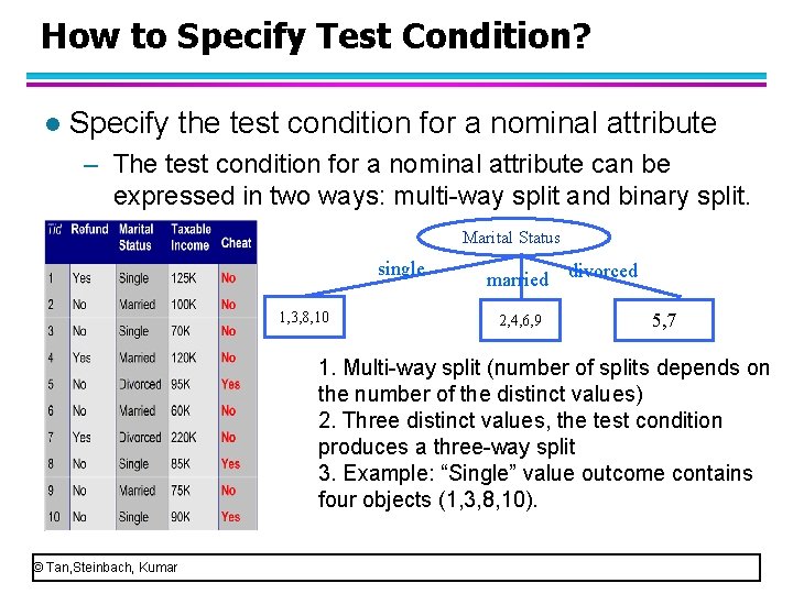
How to Specify Test Condition? l Specify the test condition for a nominal attribute – The test condition for a nominal attribute can be expressed in two ways: multi-way split and binary split. Marital Status single 1, 3, 8, 10 married divorced 2, 4, 6, 9 5, 7 1. Multi-way split (number of splits depends on the number of the distinct values) 2. Three distinct values, the test condition produces a three-way split 3. Example: “Single” value outcome contains four objects (1, 3, 8, 10). © Tan, Steinbach, Kumar

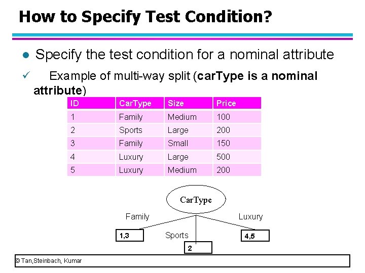
How to Specify Test Condition? Specify the test condition for a nominal attribute ü Example of multi-way split (car. Type is a nominal l attribute) ID Car. Type Size Price 1 Family Medium 100 2 Sports Large 200 3 Family Small 150 4 Luxury Large 500 5 Luxury Medium 200 Car. Type Family 1, 3 Luxury Sports 2 © Tan, Steinbach, Kumar 4, 5

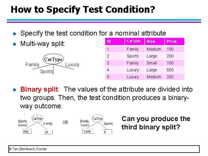
How to Specify Test Condition? l l Specify the test condition for a nominal attribute Car. Type ID Size Price Multi-way split: Car. Type Family Luxury Sports l 1 Family Medium 100 2 Sports Large 200 3 Family Small 150 4 Luxury Large 500 5 Luxury Medium 200 Binary split: The values of the attribute are divided into two groups. Then, the test condition produces a binaryway outcome. Can you produce third binary split? © Tan, Steinbach, Kumar

How to Specify Test Condition? l Specify the test condition for each attribute type – Binary – Nominal – Ordinal – Continuous l Depends on number of ways to split – 2 -way split – Multi-way split © Tan, Steinbach, Kumar

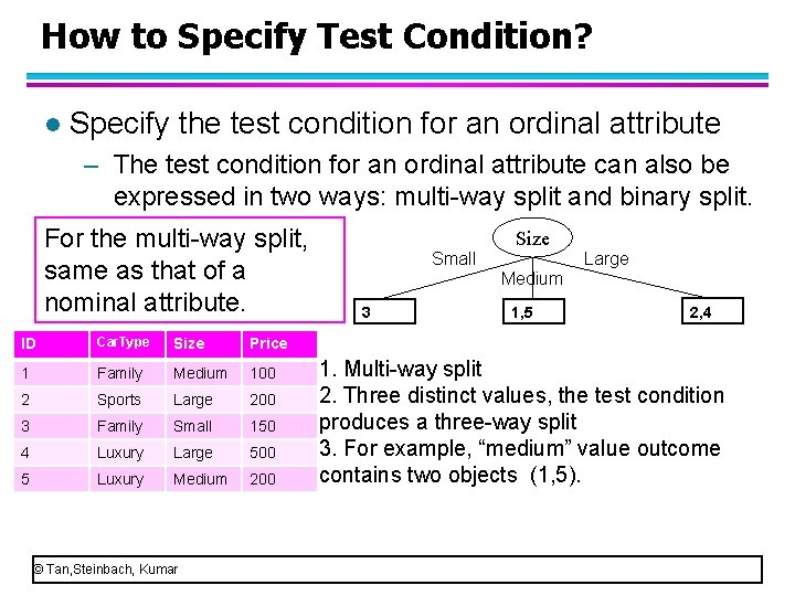
How to Specify Test Condition? l Specify the test condition for an ordinal attribute – The test condition for an ordinal attribute can also be expressed in two ways: multi-way split and binary split. For the multi-way split, same as that of a nominal attribute. ID Car. Type Size Price 1 Family Medium 100 2 Sports Large 200 3 Family Small 150 4 Luxury Large 500 5 Luxury Medium 200 © Tan, Steinbach, Kumar Size Small 3 Medium 1, 5 Large 2, 4 1. Multi-way split 2. Three distinct values, the test condition produces a three-way split 3. For example, “medium” value outcome contains two objects (1, 5).

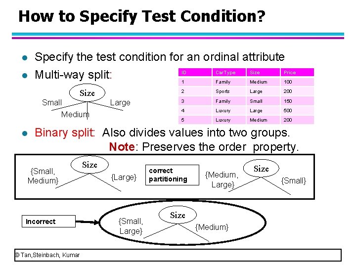
How to Specify Test Condition? l l Specify the test condition for an ordinal attribute ID Car. Type Size Price Multi-way split: 1 Family Medium 100 Size Small Medium l Large 2 Sports Large 200 3 Family Small 150 4 Luxury Large 500 5 Luxury Medium 200 Binary split: Also divides values into two groups. Note: Preserves the order property. {Small, Medium} Size Incorrect © Tan, Steinbach, Kumar {Large} {Small, Large} correct partitioning {Medium, Large} Size {Medium} Size {Small}

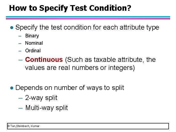
How to Specify Test Condition? l Specify the test condition for each attribute type – Binary – Nominal – Ordinal – Continuous (Such as taxable attribute, the values are real numbers or integers) l Depends on number of ways to split – 2 -way split – Multi-way split © Tan, Steinbach, Kumar

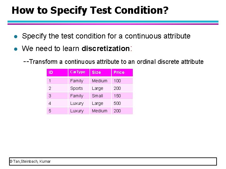
How to Specify Test Condition? l Specify the test condition for a continuous attribute l We need to learn discretization: --Transform a continuous attribute to an ordinal discrete attribute ID Car. Type Size Price 1 Family Medium 100 2 Sports Large 200 3 Family Small 150 4 Luxury Large 500 5 Luxury Medium 200 © Tan, Steinbach, Kumar

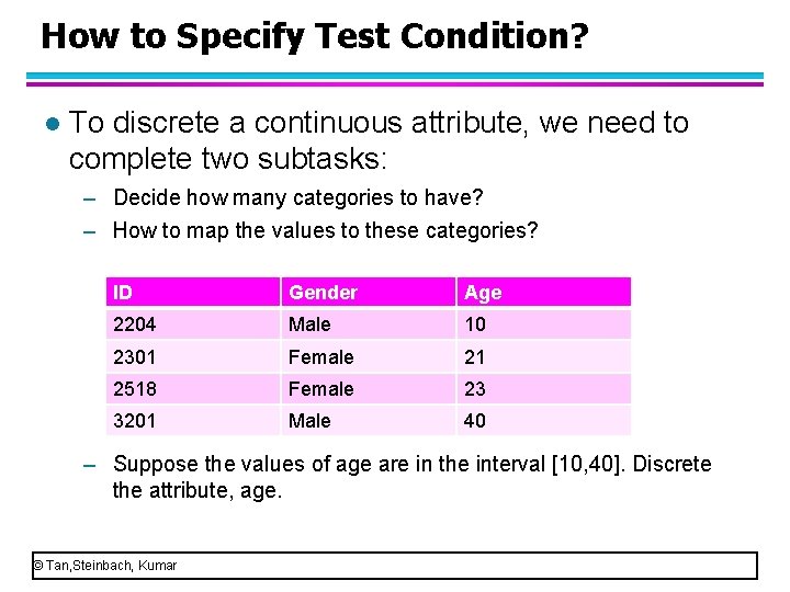
How to Specify Test Condition? l To discrete a continuous attribute, we need to complete two subtasks: – Decide how many categories to have? – How to map the values to these categories? ID Gender Age 2204 Male 10 2301 Female 21 2518 Female 23 3201 Male 40 – Suppose the values of age are in the interval [10, 40]. Discrete the attribute, age. © Tan, Steinbach, Kumar

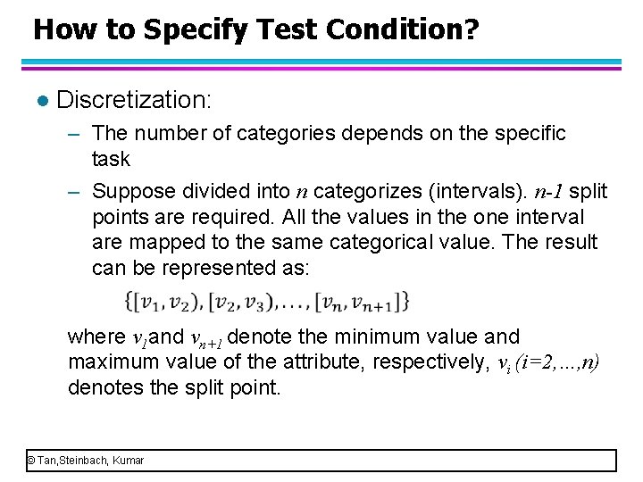
How to Specify Test Condition? l Discretization: – The number of categories depends on the specific task – Suppose divided into n categorizes (intervals). n-1 split points are required. All the values in the one interval are mapped to the same categorical value. The result can be represented as: where v 1 and vn+1 denote the minimum value and maximum value of the attribute, respectively, vi (i=2, …, n) denotes the split point. © Tan, Steinbach, Kumar

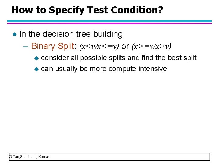
How to Specify Test Condition? l Discretization: – Suppose Age is in [10, 40], and 2 categorizes. – Common approaches: (1) The equal width approach: each interval has the same width. [10, 25), [25, 40] (2) The equal frequency approach: each interval has the same number of objects. [10, 22), [22, 40] It is also called “binary split” when the attribute is transformed to two categorizes. Suppose v is the split point, a binary split can be l expressed as (x<v/x<=v) or (x>=v/x>v). © Tan, Steinbach, Kumar

How to Specify Test Condition? l In the decision tree building – Binary Split: (x<v/x<=v) or (x>=v/x>v) u consider all possible splits and find the best split u can usually be more compute intensive © Tan, Steinbach, Kumar

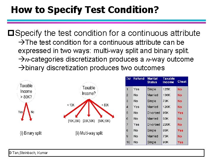
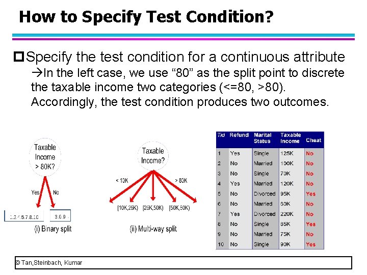
How to Specify Test Condition? p. Specify the test condition for a continuous attribute The test condition for a continuous attribute can be expressed in two ways: multi-way split and binary split. n-categories discretization produces a n-way outcome binary discretization produces two outcomes © Tan, Steinbach, Kumar

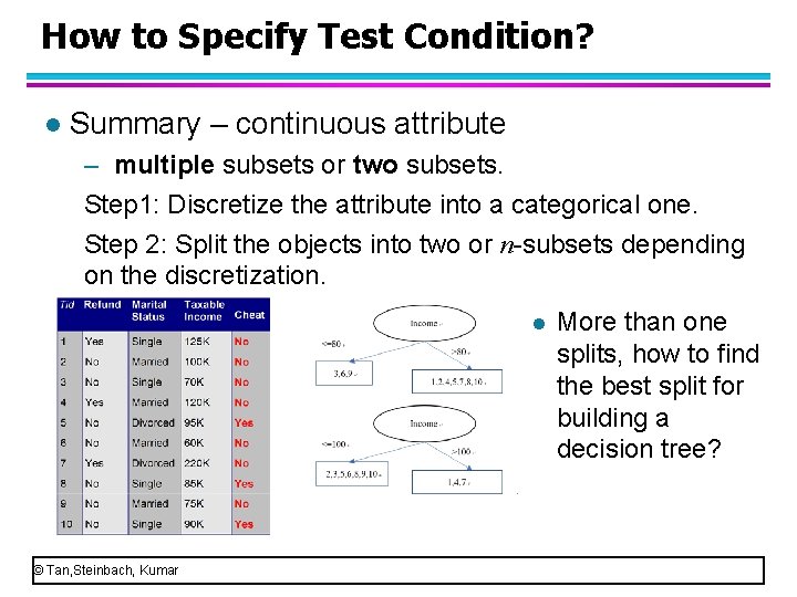
How to Specify Test Condition? p. Specify the test condition for a continuous attribute In the left case, we use “ 80” as the split point to discrete the taxable income two categories (<=80, >80). Accordingly, the test condition produces two outcomes. © Tan, Steinbach, Kumar

How to Specify Test Condition? p. Specify the test condition for a continuous attribute In the right case, we use “ 10”, “ 25”, “ 50”, “ 80” as the split points to discrete the taxable income five categories. Accordingly, the test condition produces five outcomes. © Tan, Steinbach, Kumar

How to Specify Test Condition? l Summary: specify the test condition for each attribute type – Binary – Nominal – Ordinal – Continuous © Tan, Steinbach, Kumar

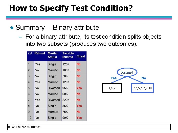
How to Specify Test Condition? l Summary – Binary attribute – For a binary attribute, its test condition splits objects into two subsets (produces two outcomes). Refund Yes 1, 4, 7 © Tan, Steinbach, Kumar No 2, 3, 5, 6, 8, 9, 10

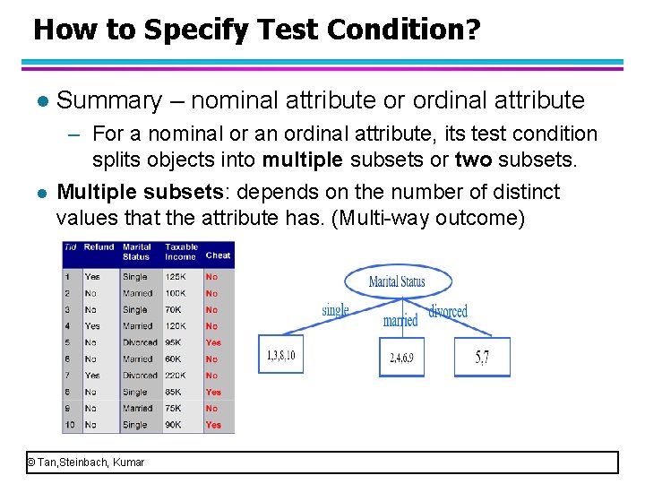
How to Specify Test Condition? l l Summary – nominal attribute or ordinal attribute – For a nominal or an ordinal attribute, its test condition splits objects into multiple subsets or two subsets. Multiple subsets: depends on the number of distinct values that the attribute has. (Multi-way outcome) © Tan, Steinbach, Kumar

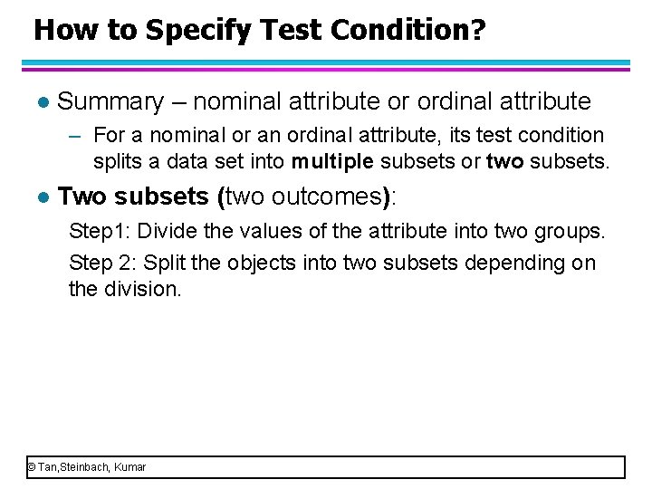
How to Specify Test Condition? l Summary – nominal attribute or ordinal attribute – For a nominal or an ordinal attribute, its test condition splits a data set into multiple subsets or two subsets. l Two subsets (two outcomes): Step 1: Divide the values of the attribute into two groups. Step 2: Split the objects into two subsets depending on the division. © Tan, Steinbach, Kumar

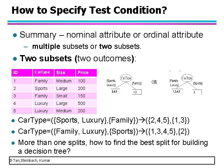
How to Specify Test Condition? l Summary – nominal attribute or ordinal attribute – multiple subsets or two subsets. l ID Two subsets (two outcomes): Car. Type Size Price 1 Family Medium 100 2 Sports Large 200 3 Family Small 150 4 Luxury Large 500 5 Luxury Medium 200 Car. Type=({Sports, Luxury}, {Family}) ({2, 4, 5}, {1, 3}) l Car. Type=({Family, Luxury}, {Sports}) ({1, 3, 4, 5}, {2}) l More than one splits, how to find the best split for building a decision tree? © Tan, Steinbach, Kumar l

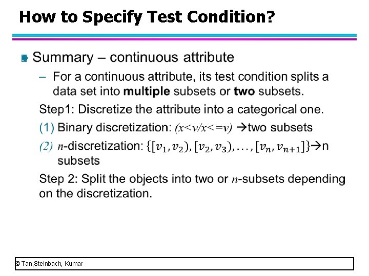
How to Specify Test Condition? l © Tan, Steinbach, Kumar

How to Specify Test Condition? l Summary – continuous attribute – multiple subsets or two subsets. Step 1: Discretize the attribute into a categorical one. Step 2: Split the objects into two or n-subsets depending on the discretization. l More than one splits, how to find the best split for building a decision tree? © Tan, Steinbach, Kumar

Tree Induction l Issues – Determine how to split the records u. How to specify the attribute test condition? u. How to determine the best split? – Determine when to stop splitting l From the above discussion, an attribute can have more than one splits for objects. But which split is the best? © Tan, Steinbach, Kumar

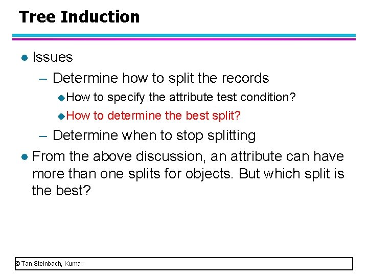
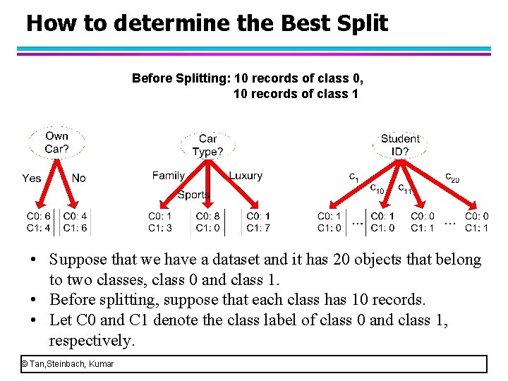
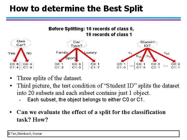
How to determine the Best Split Before Splitting: 10 records of class 0, 10 records of class 1 • Suppose that we have a dataset and it has 20 objects that belong to two classes, class 0 and class 1. • Before splitting, suppose that each class has 10 records. • Let C 0 and C 1 denote the class label of class 0 and class 1, respectively. © Tan, Steinbach, Kumar

How to determine the Best Split Before Splitting: 10 records of class 0, 10 records of class 1 • Three splits of the dataset. • First picture, the test condition of “Own Car” splits the dataset into two subsets and each subset has 10 objects. • Left subset, 6 records belong to C 0 and 4 records belong to C 1. • Right subset, 4 records belong to C 0 and 6 records belong to C 1. Just as the test condition of “refund” splits the dataset into two subsets. In the first subset, there are three objects that belong to “No”. In the left subset, there are 7 objects, four of which belong to “No” and three of which belong to “Yes”. © Tan, Steinbach, Kumar

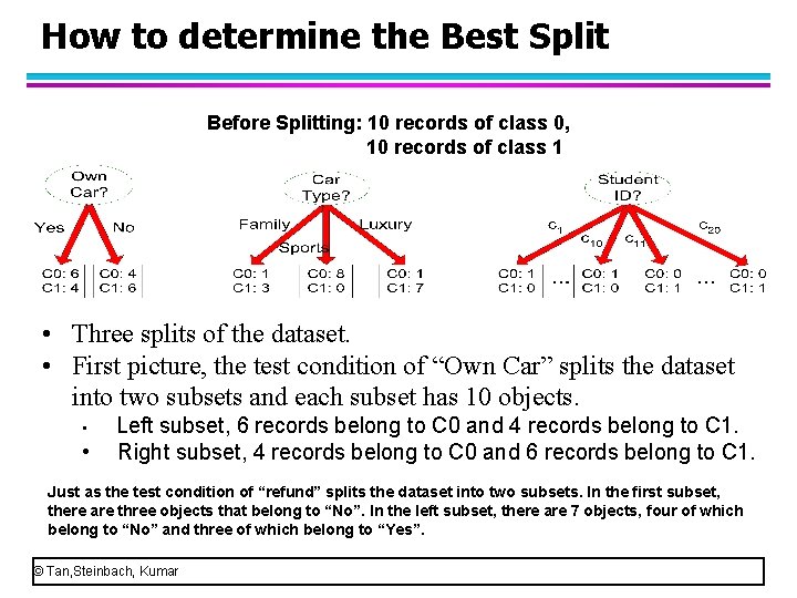
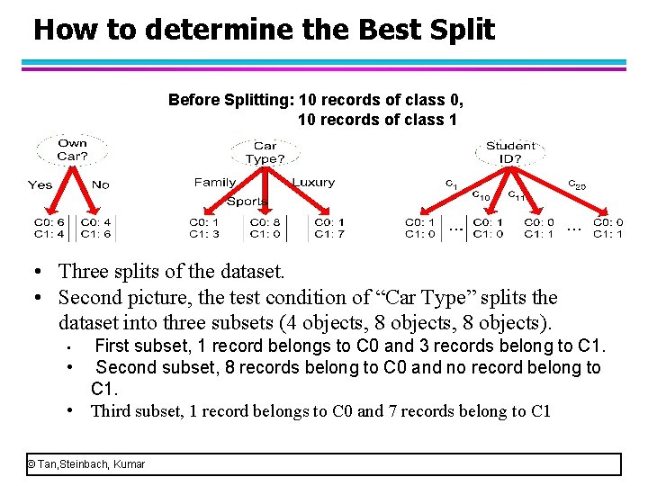
How to determine the Best Split Before Splitting: 10 records of class 0, 10 records of class 1 • Three splits of the dataset. • Second picture, the test condition of “Car Type” splits the dataset into three subsets (4 objects, 8 objects). • First subset, 1 record belongs to C 0 and 3 records belong to C 1. • Second subset, 8 records belong to C 0 and no record belong to C 1. • Third subset, 1 record belongs to C 0 and 7 records belong to C 1 © Tan, Steinbach, Kumar

How to determine the Best Split Before Splitting: 10 records of class 0, 10 records of class 1 • Three splits of the dataset. • Third picture, the test condition of “Student ID” splits the dataset into 20 subsets and each subset contains just 1 object. • Each subset, the object belongs to either C 0 or C 1. • Can we evaluate the effect of a split for the classification task? How? © Tan, Steinbach, Kumar

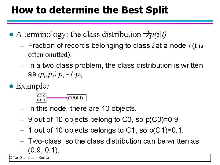
How to determine the Best Split l A terminology: the class distribution p(i|t) – Fraction of records belonging to class i at a node t (t is often omitted). – In a two-class problem, the class distribution is written as (p 0, p 1) p 1=1 -p 0. l Example: – – In this node, there are 10 objects. 9 out of 10 objects belong to C 0, so p(C 0)=0. 9; 1 out of 10 objects belongs to C 1, so p(C 1)=0. 1. Two-class, so the class distribution can be written as (0. 9, 0. 1). © Tan, Steinbach, Kumar

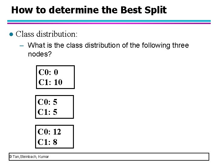
How to determine the Best Split l Class distribution: – What is the class distribution of the following three nodes? C 0: 0 C 1: 10 C 0: 5 C 1: 5 C 0: 12 C 1: 8 © Tan, Steinbach, Kumar

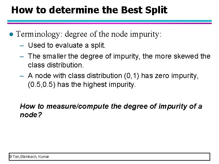
How to determine the Best Split l Terminology: degree of the node impurity: – Used to evaluate a split. – The smaller the degree of impurity, the more skewed the class distribution. – A node with class distribution (0, 1) has zero impurity, (0. 5, 0. 5) has the highest impurity. How to measure/compute the degree of impurity of a node? © Tan, Steinbach, Kumar

Measures of Node Impurity l Gini Index l Entropy l Classification error © Tan, Steinbach, Kumar

Measures of Node Impurity l Gini Index l Entropy l Classification error © Tan, Steinbach, Kumar

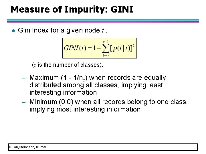
Measure of Impurity: GINI l Gini Index for a given node t : (c is the number of classes). – Maximum (1 - 1/nc) when records are equally distributed among all classes, implying least interesting information – Minimum (0. 0) when all records belong to one class, implying most interesting information © Tan, Steinbach, Kumar

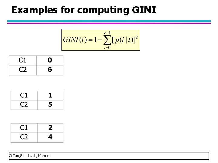
Examples for computing GINI © Tan, Steinbach, Kumar

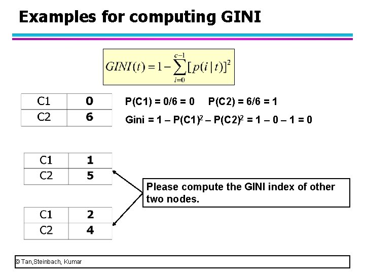
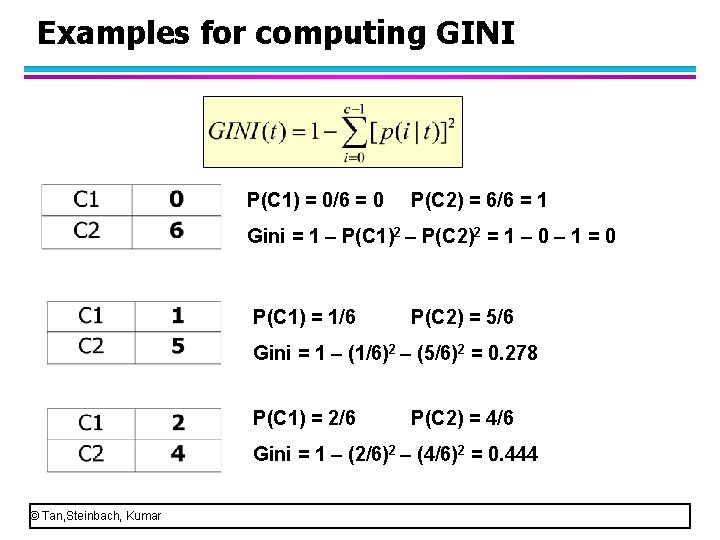
Examples for computing GINI P(C 1) = 0/6 = 0 P(C 2) = 6/6 = 1 Gini = 1 – P(C 1)2 – P(C 2)2 = 1 – 0 – 1 = 0 Please compute the GINI index of other two nodes. © Tan, Steinbach, Kumar

Examples for computing GINI P(C 1) = 0/6 = 0 P(C 2) = 6/6 = 1 Gini = 1 – P(C 1)2 – P(C 2)2 = 1 – 0 – 1 = 0 P(C 1) = 1/6 P(C 2) = 5/6 Gini = 1 – (1/6)2 – (5/6)2 = 0. 278 P(C 1) = 2/6 P(C 2) = 4/6 Gini = 1 – (2/6)2 – (4/6)2 = 0. 444 © Tan, Steinbach, Kumar

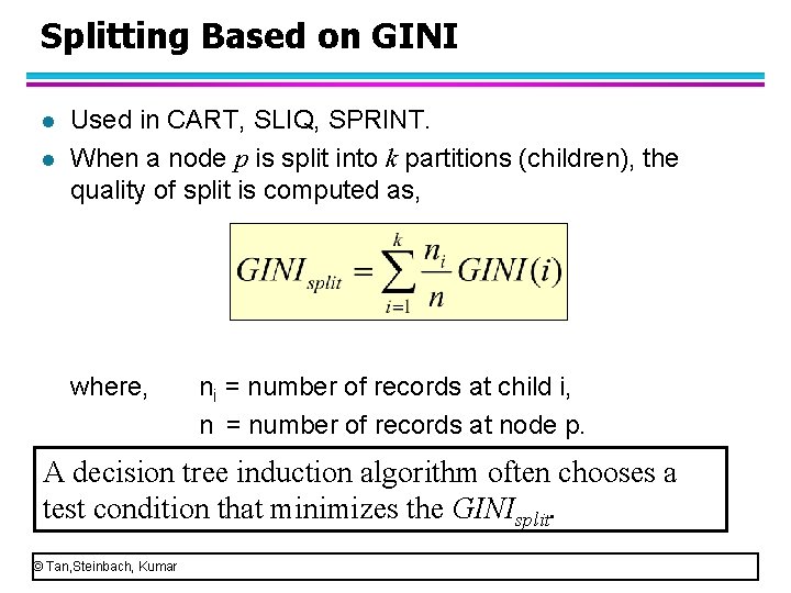
Splitting Based on GINI l l Used in CART, SLIQ, SPRINT. When a node p is split into k partitions (children), the quality of split is computed as, where, ni = number of records at child i, n = number of records at node p. A decision tree induction algorithm often chooses a test condition that minimizes the GINIsplit. © Tan, Steinbach, Kumar

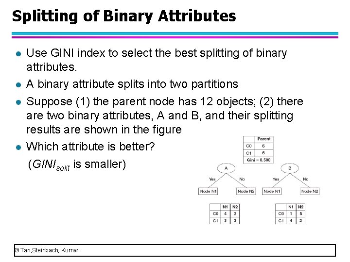
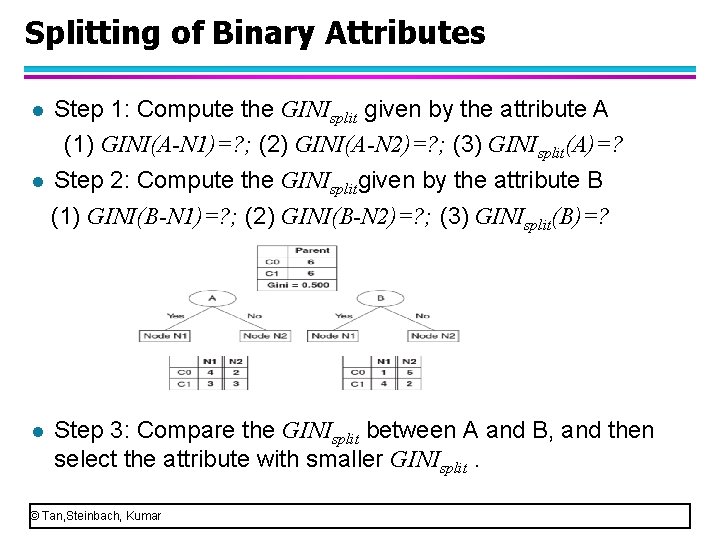
Splitting of Binary Attributes Use GINI index to select the best splitting of binary attributes. l A binary attribute splits into two partitions l Suppose (1) the parent node has 12 objects; (2) there are two binary attributes, A and B, and their splitting results are shown in the figure l Which attribute is better? (GINIsplit is smaller) l © Tan, Steinbach, Kumar

Splitting of Binary Attributes Step 1: Compute the GINIsplit given by the attribute A (1) GINI(A-N 1)=? ; (2) GINI(A-N 2)=? ; (3) GINIsplit(A)=? l Step 2: Compute the GINIsplitgiven by the attribute B (1) GINI(B-N 1)=? ; (2) GINI(B-N 2)=? ; (3) GINIsplit(B)=? l l Step 3: Compare the GINIsplit between A and B, and then select the attribute with smaller GINIsplit. © Tan, Steinbach, Kumar

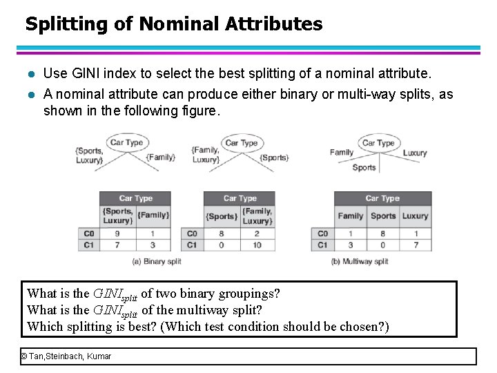
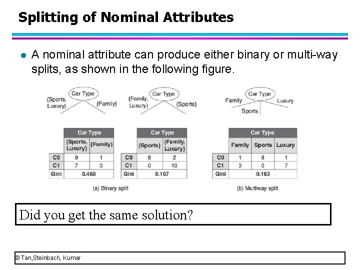
Splitting of Nominal Attributes l Use GINI index to select the best splitting of a nominal attribute. l A nominal attribute can produce either binary or multi-way splits, as shown in the following figure. What is the GINIsplit of two binary groupings? What is the GINIsplit of the multiway split? Which splitting is best? (Which test condition should be chosen? ) © Tan, Steinbach, Kumar

Splitting of Nominal Attributes l A nominal attribute can produce either binary or multi-way splits, as shown in the following figure. Did you get the same solution? © Tan, Steinbach, Kumar

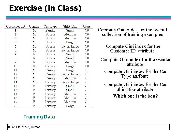
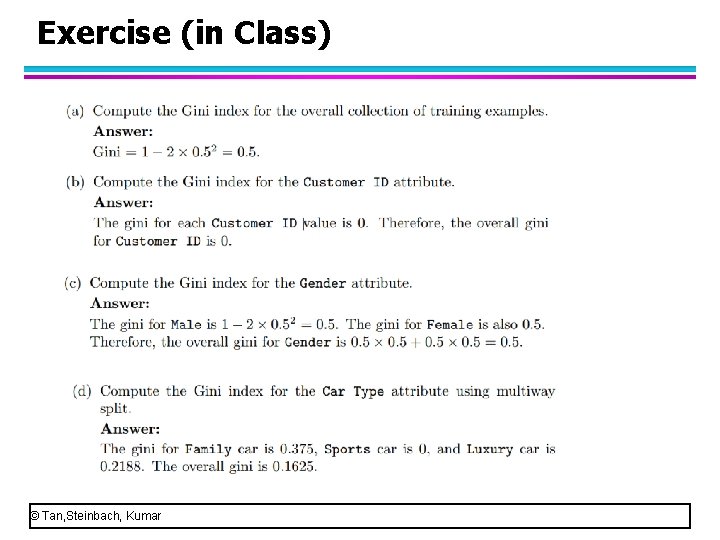
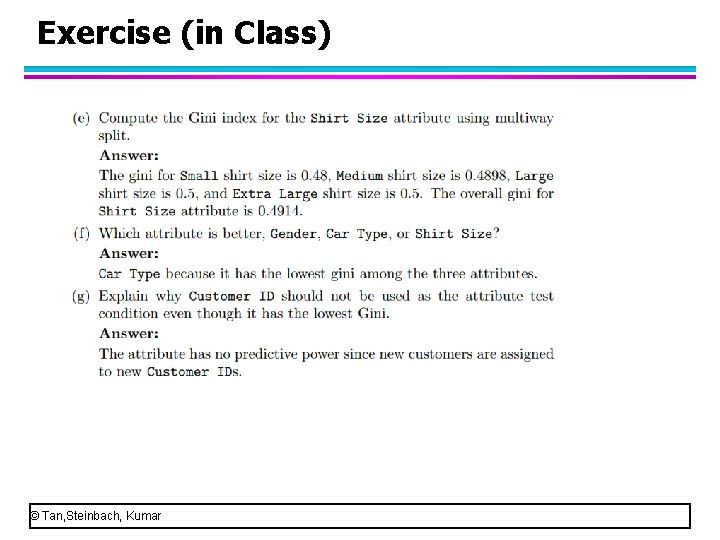
Exercise (in Class) Compute Gini index for the overall collection of training examples Compute Gini index for the Customer ID attribute Compute Gini index for the Gender attribute Compute Gini index for the Car Type attribute Compute Gini index for the Car Shirt Size attribute Which one is the best? Training Data © Tan, Steinbach, Kumar

Exercise (in Class) © Tan, Steinbach, Kumar

Exercise (in Class) © Tan, Steinbach, Kumar

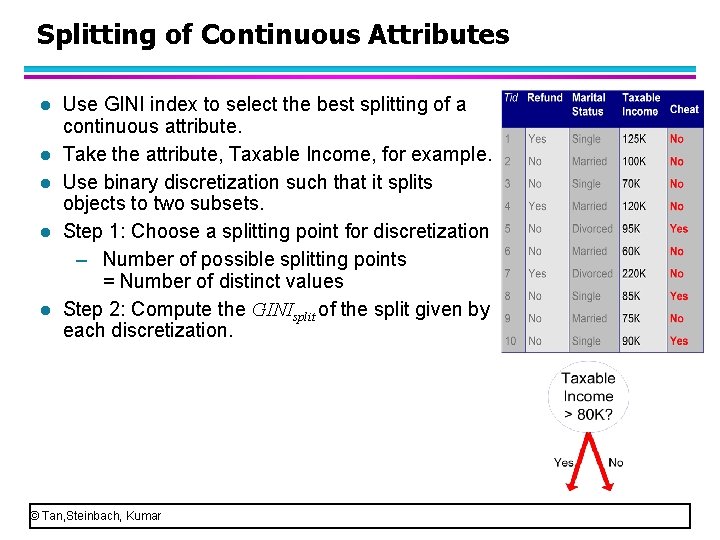
Splitting of Continuous Attributes l l l Use GINI index to select the best splitting of a continuous attribute. Take the attribute, Taxable Income, for example. Use binary discretization such that it splits objects to two subsets. Step 1: Choose a splitting point for discretization – Number of possible splitting points = Number of distinct values Step 2: Compute the GINIsplit of the split given by each discretization. © Tan, Steinbach, Kumar

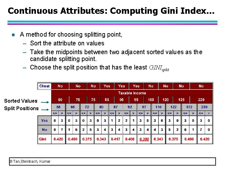
Continuous Attributes: Computing Gini Index. . . l A method for choosing splitting point, – Sort the attribute on values – Take the midpoints between two adjacent sorted values as the candidate splitting point. – Choose the split position that has the least GINIsplit Sorted Values Split Positions © Tan, Steinbach, Kumar

Tree Induction l Greedy strategy. – Split the records based on an attribute test that optimizes certain criterion. l Issues – Determine how to split the records u. How to specify the attribute test condition? u. How to determine the best split? – Determine when to stop splitting © Tan, Steinbach, Kumar

Stopping Criteria for Tree Induction l Stop expanding a node when all the records belong to the same class l Stop expanding a node when all the records have similar attribute values l Early termination © Tan, Steinbach, Kumar

Decision Tree Classification Task Decision Tree © Tan, Steinbach, Kumar

Apply Model to Test Data Start from the root of tree. Refund Yes No NO Mar. St Single, Divorced Tax. Inc < 80 K NO © Tan, Steinbach, Kumar Married NO > 80 K YES

Apply Model to Test Data Refund Yes No NO Mar. St Single, Divorced Tax. Inc < 80 K NO © Tan, Steinbach, Kumar Married NO > 80 K YES

Apply Model to Test Data Refund Yes No NO Mar. St Single, Divorced Tax. Inc < 80 K NO © Tan, Steinbach, Kumar Married NO > 80 K YES

Apply Model to Test Data Refund Yes No NO Mar. St Single, Divorced Tax. Inc < 80 K NO © Tan, Steinbach, Kumar Married NO > 80 K YES

Apply Model to Test Data Refund Yes No NO Mar. St Single, Divorced Tax. Inc < 80 K NO © Tan, Steinbach, Kumar Married NO > 80 K YES

Apply Model to Test Data Refund Yes No NO Mar. St Single, Divorced Tax. Inc < 80 K NO © Tan, Steinbach, Kumar Married NO > 80 K YES Assign Cheat to “No”

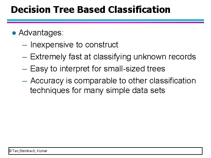
Decision Tree Based Classification l Advantages: – Inexpensive to construct – Extremely fast at classifying unknown records – Easy to interpret for small-sized trees – Accuracy is comparable to other classification techniques for many simple data sets © Tan, Steinbach, Kumar

Other Issues Data Fragmentation l Search Strategy l Expressiveness l Tree Replication l © Tan, Steinbach, Kumar

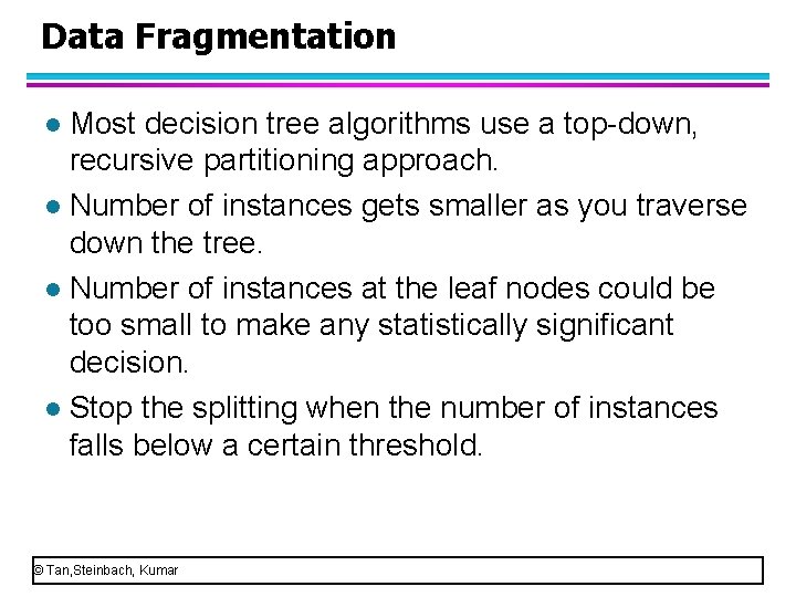
Data Fragmentation Most decision tree algorithms use a top-down, recursive partitioning approach. l Number of instances gets smaller as you traverse down the tree. l Number of instances at the leaf nodes could be too small to make any statistically significant decision. l Stop the splitting when the number of instances falls below a certain threshold. l © Tan, Steinbach, Kumar

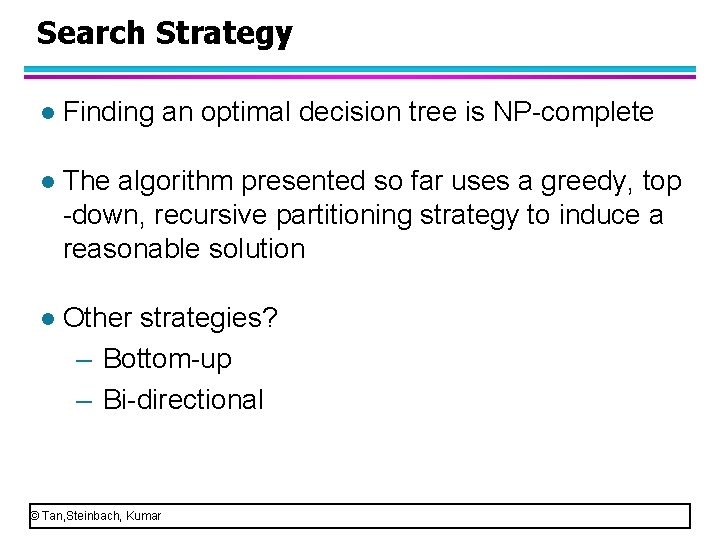
Search Strategy l Finding an optimal decision tree is NP-complete l The algorithm presented so far uses a greedy, top -down, recursive partitioning strategy to induce a reasonable solution l Other strategies? – Bottom-up – Bi-directional © Tan, Steinbach, Kumar

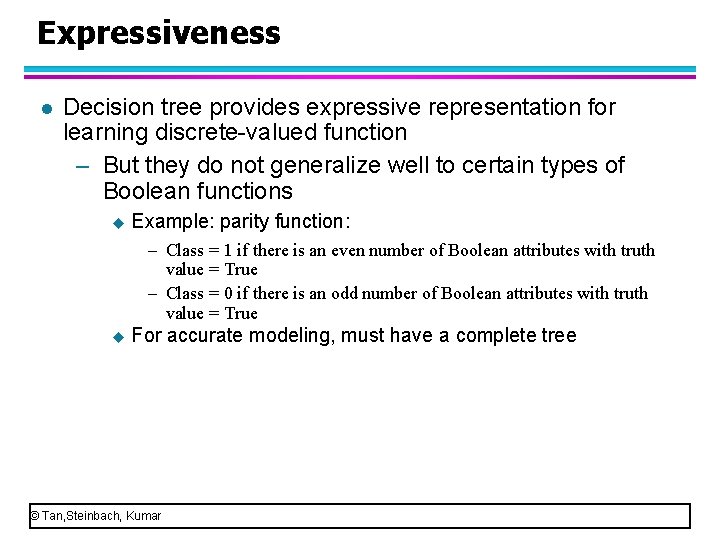
Expressiveness l Decision tree provides expressive representation for learning discrete-valued function – But they do not generalize well to certain types of Boolean functions u Example: parity function: – Class = 1 if there is an even number of Boolean attributes with truth value = True – Class = 0 if there is an odd number of Boolean attributes with truth value = True u For accurate modeling, must have a complete tree © Tan, Steinbach, Kumar

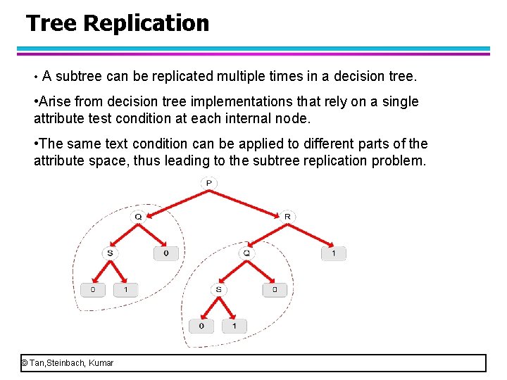
Tree Replication • A subtree can be replicated multiple times in a decision tree. • Arise from decision tree implementations that rely on a single attribute test condition at each internal node. • The same text condition can be applied to different parts of the attribute space, thus leading to the subtree replication problem. © Tan, Steinbach, Kumar

Other Issues Data Fragmentation l Search Strategy l Expressiveness l Tree Replication l Many researches have been done to solve these issues. © Tan, Steinbach, Kumar

Classification Concepts l Section 1: Decision Tree l. Section 2: Model Overfitting © Tan, Steinbach, Kumar

Model Overfitting and Underfitting l Concept of Overfitting and Underfitting l Causes of model overfitting l Estimation of generalization errors l Address overfitting © Tan, Steinbach, Kumar

Model Overfitting and Underfitting l Two kinds of errors of a classification model: training error and generalization error • Training error: the number of misclassification errors committed on training records. Generalization error: the expected error of the model on previously unseen records. A good classification model must have low training error as well as low generalization error. • l © Tan, Steinbach, Kumar

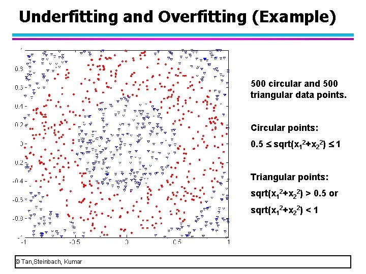
Underfitting and Overfitting (Example) 500 circular and 500 triangular data points. Circular points: 0. 5 sqrt(x 12+x 22) 1 Triangular points: sqrt(x 12+x 22) > 0. 5 or sqrt(x 12+x 22) < 1 © Tan, Steinbach, Kumar

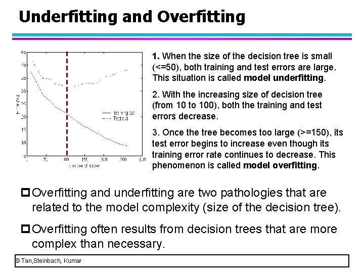
Underfitting and Overfitting 1. When the size of the decision tree is small (<=50), both training and test errors are large. This situation is called model underfitting. 2. With the increasing size of decision tree (from 10 to 100), both the training and test errors decrease. 3. Once the tree becomes too large (>=150), its test error begins to increase even though its training error rate continues to decrease. This phenomenon is called model overfitting. p. Overfitting and underfitting are two pathologies that are related to the model complexity (size of the decision tree). p. Overfitting often results from decision trees that are more complex than necessary. © Tan, Steinbach, Kumar

Model Overfitting and Underfitting l Understand overfitting • The training error of a model can be reduced by increasing the model complexity. For example, the leaf nodes can be expanded until it perfectly fits the training data. In this case, the training error is zero, however, the test error can be large because the tree may contain nodes that accidently fit some of noise points in the training data. Such nodes can degrade the performance of the tree because they do not generalize well to the test objects. • © Tan, Steinbach, Kumar

Model Overfitting and Underfitting l Common causes of model overfitting • Noise samples. • Lack of representative samples. • Multiple comparison procedure. © Tan, Steinbach, Kumar

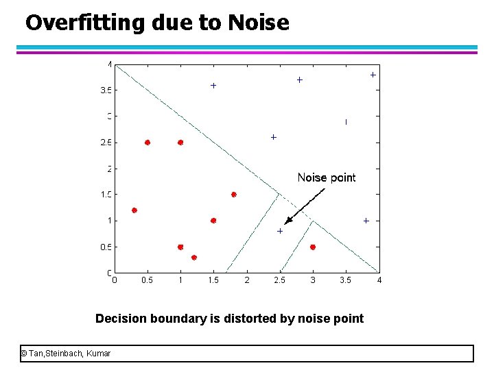
Overfitting due to Noise Decision boundary is distorted by noise point © Tan, Steinbach, Kumar

Estimation of generalization errors p A good model: low training error as well as low generalization error. p Only a low training error cannot indicate that a classification model is good. p We need to estimate the generalization error such that we can evaluate a classification model for generalization. © Tan, Steinbach, Kumar

Estimating Generalization Errors l Common estimation methods • Using training errors to estimate • Pessimistic approach • Estimating statistical bounds • Using a validation set © Tan, Steinbach, Kumar

Estimating Generalization Errors l Using a validation set: – The original training data set is divided into two smaller subsets: training subset and validation subset. – Training subset is used to build a classification model. – The validation subset is used to estimate the generalization error. – Typically, two-thirds as training subset, while remaining one-third as validation subset. © Tan, Steinbach, Kumar

How to Address Overfitting… l Some techniques have been proposed to address overfitting such as prepruning and post-pruning © Tan, Steinbach, Kumar

Classification Concepts Section 1: Decision Tree Section 2: Model Overfitting l l l. Section 3: Model Evaluation © Tan, Steinbach, Kumar

Model Evaluation l Metrics for Performance Evaluation – How to evaluate the performance of a classification model? © Tan, Steinbach, Kumar

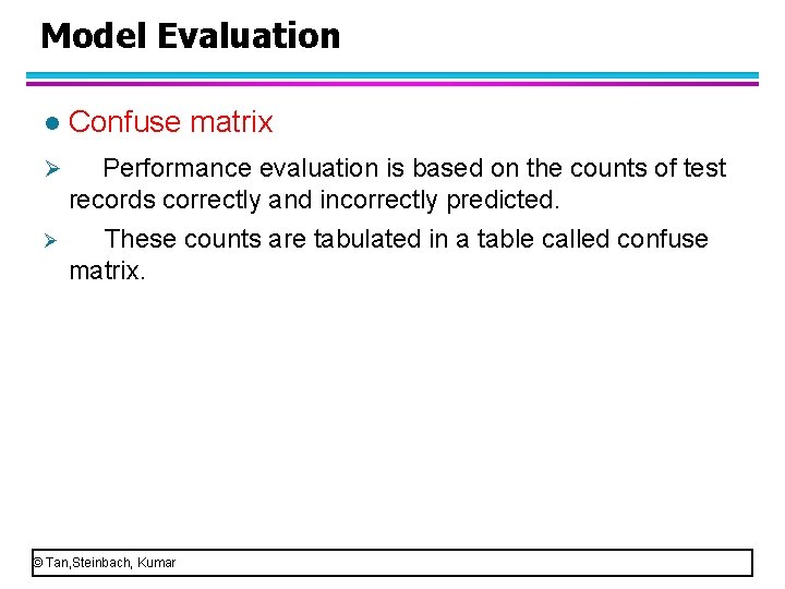
Model Evaluation Confuse matrix Ø Performance evaluation is based on the counts of test l Ø records correctly and incorrectly predicted. These counts are tabulated in a table called confuse matrix. © Tan, Steinbach, Kumar

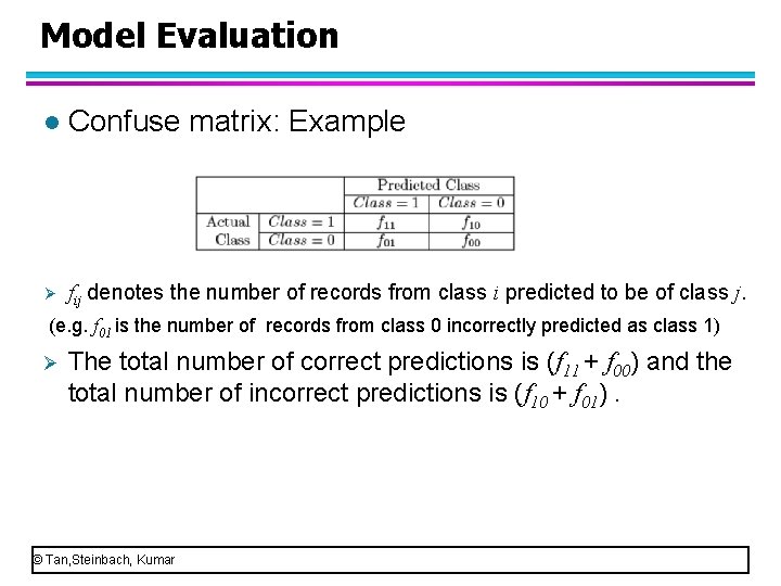
Model Evaluation l Confuse matrix: Example Ø fij denotes the number of records from class i predicted to be of class j. (e. g. f 01 is the number of records from class 0 incorrectly predicted as class 1) Ø The total number of correct predictions is (f 11 + f 00) and the total number of incorrect predictions is (f 10 + f 01). © Tan, Steinbach, Kumar

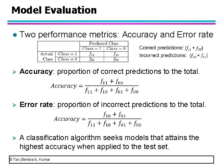
Model Evaluation l Two performance metrics: Accuracy and Error rate Ø Accuracy: proportion of correct predictions to the total. Ø Error rate: proportion of incorrect predictions to the total. Ø A classification algorithm seeks models that attains the highest accuracy when applied to the test set. © Tan, Steinbach, Kumar

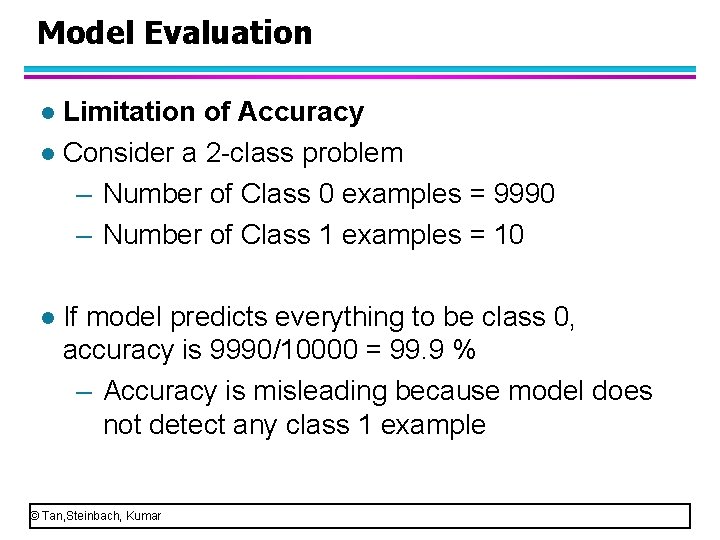
Model Evaluation Limitation of Accuracy l Consider a 2 -class problem – Number of Class 0 examples = 9990 – Number of Class 1 examples = 10 l l If model predicts everything to be class 0, accuracy is 9990/10000 = 99. 9 % – Accuracy is misleading because model does not detect any class 1 example © Tan, Steinbach, Kumar

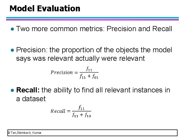
Model Evaluation l Two more common metrics: Precision and Recall l Precision: the proportion of the objects the model says was relevant actually were relevant l Recall: the ability to find all relevant instances in a dataset © Tan, Steinbach, Kumar

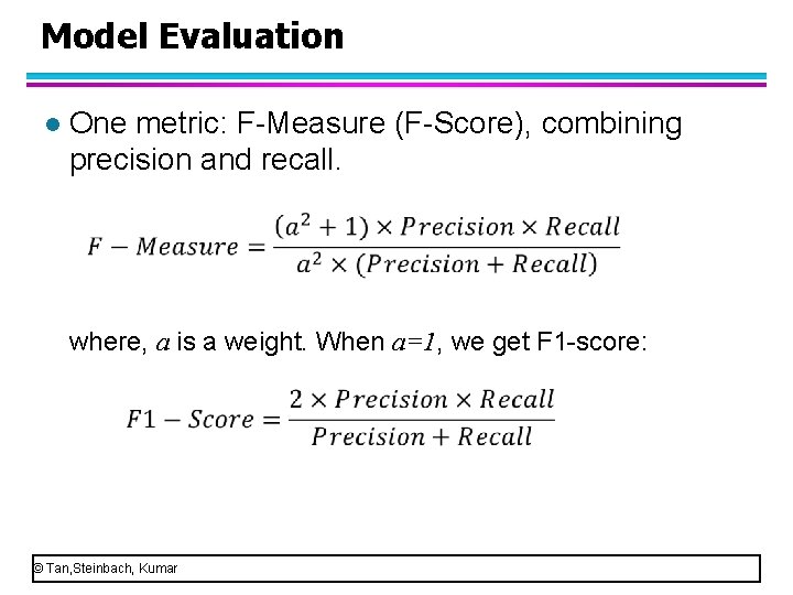
Model Evaluation l One metric: F-Measure (F-Score), combining precision and recall. where, a is a weight. When a=1, we get F 1 -score: © Tan, Steinbach, Kumar