Data Science 100 Lecture 7 Modeling and Estimation

Data Science 100 Lecture 7: Modeling and Estimation Slides by: Joseph E. Gonzalez, jegonzal@berkeley. edu 2018 updates - Fernando Perez, fernando. perez@berkele. edu ?

Recap … so far we have covered Ø Data collection: Surveys, sampling, administrative data Ø Data cleaning and manipulation: Pandas, text & regexes. Ø Exploratory Data Analysis Ø Joining and grouping data Ø Structure, Granularity, Temporality, Faithfulness and Scope Ø Basic exploratory data visualization Ø Data Visualization: Ø Kinds of visualizations and the use of size, area, and color Ø Data transformations using Tukey Mosteller bulge diagram Ø An introduction to database systems and SQL

Today – Models & Estimation

What is a model?

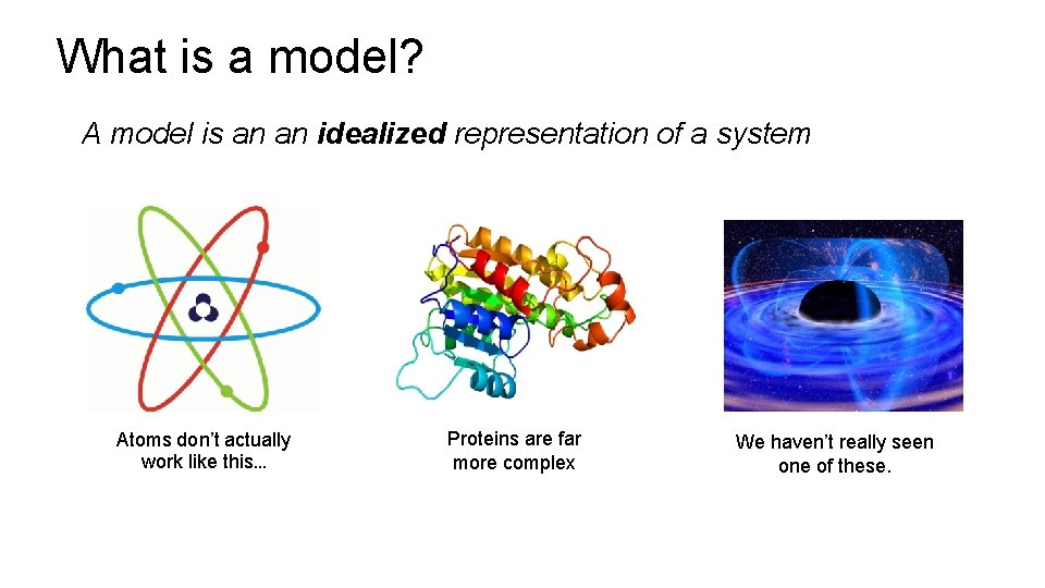
What is a model? A model is an an idealized representation of a system Atoms don’t actually work like this… Proteins are far more complex We haven’t really seen one of these.

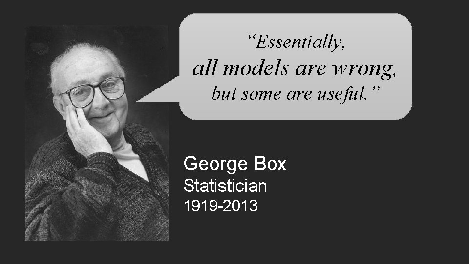
“Essentially, all models are wrong, but some are useful. ” George Box Statistician 1919 -2013

Why do we build models?

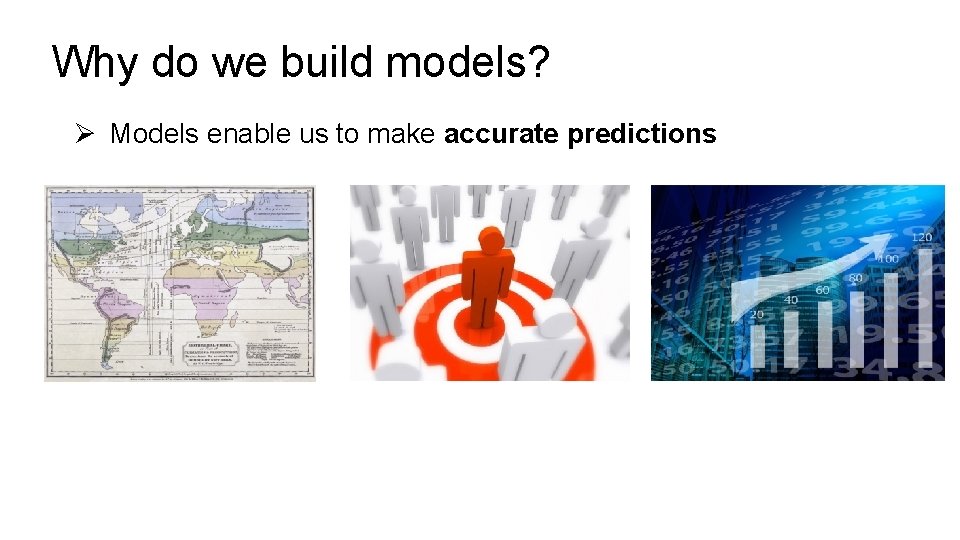
Why do we build models? Ø Models enable us to make accurate predictions

Ø Provide insight into complex phenomena

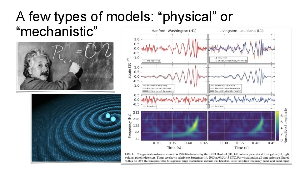
A few types of models: “physical” or “mechanistic”

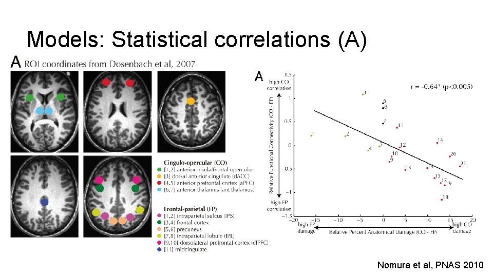
Models: Statistical correlations (A) Nomura et al, PNAS 2010

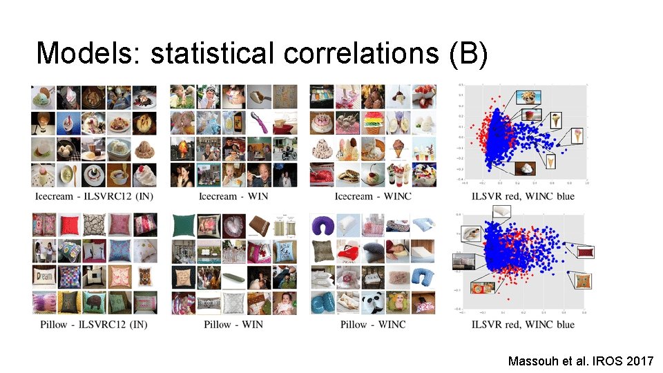
Models: statistical correlations (B) Massouh et al. IROS 2017

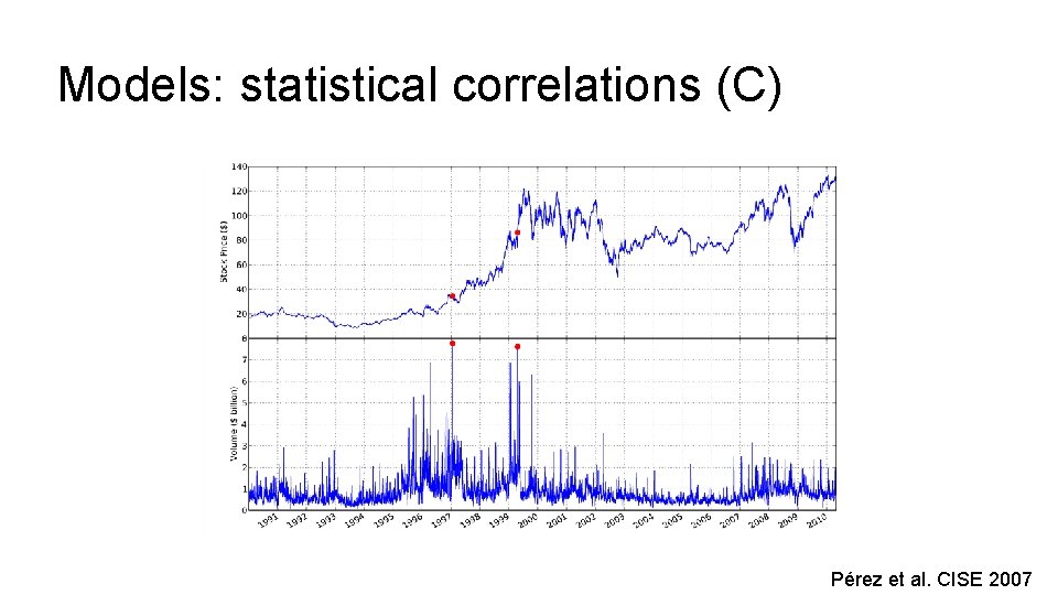
Models: statistical correlations (C) Pérez et al. CISE 2007

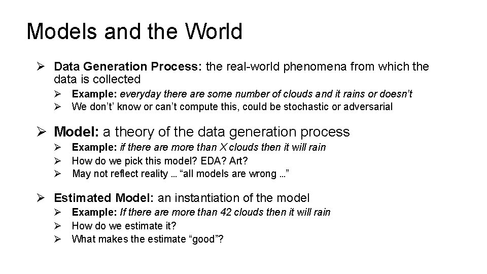
Models and the World Ø Data Generation Process: the real-world phenomena from which the data is collected Ø Example: everyday there are some number of clouds and it rains or doesn’t Ø We don’t’ know or can’t compute this, could be stochastic or adversarial Ø Model: a theory of the data generation process Ø Example: if there are more than X clouds then it will rain Ø How do we pick this model? EDA? Art? Ø May not reflect reality … “all models are wrong …” Ø Estimated Model: an instantiation of the model Ø Example: If there are more than 42 clouds then it will rain Ø How do we estimate it? Ø What makes the estimate “good”?

Example – Restaurant Tips Follow along with the notebook …

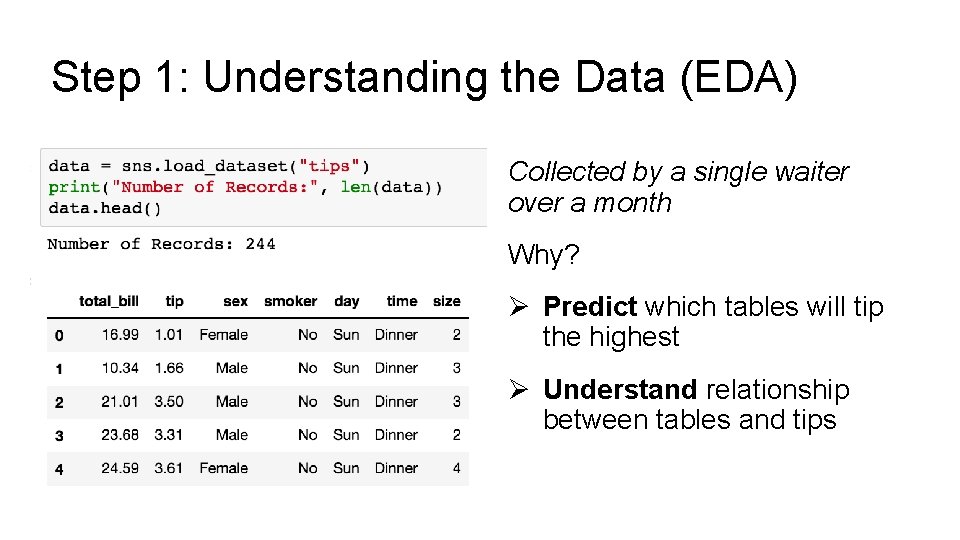
Step 1: Understanding the Data (EDA) Collected by a single waiter over a month Why? Ø Predict which tables will tip the highest Ø Understand relationship between tables and tips

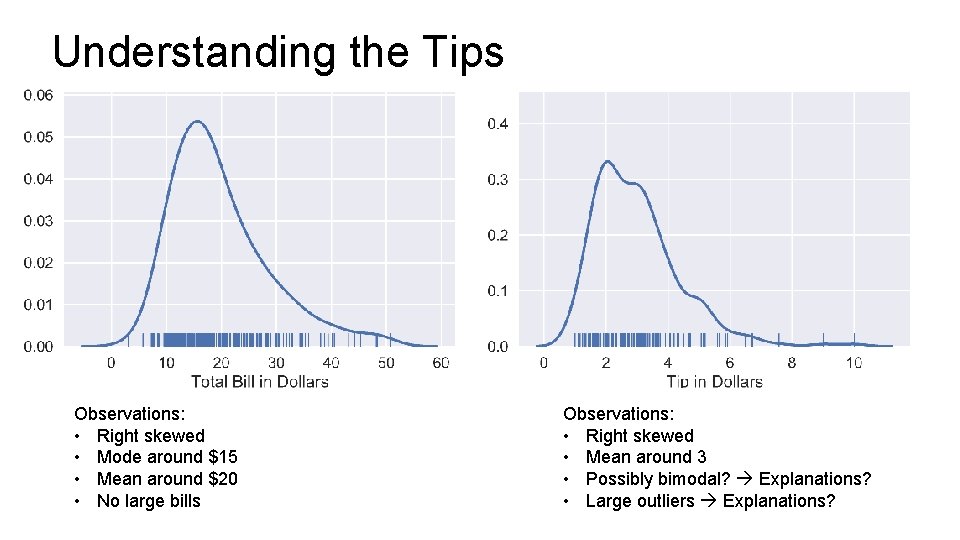
Understanding the Tips Observations: • Right skewed • Mode around $15 • Mean around $20 • No large bills Observations: • Right skewed • Mean around 3 • Possibly bimodal? Explanations? • Large outliers Explanations?

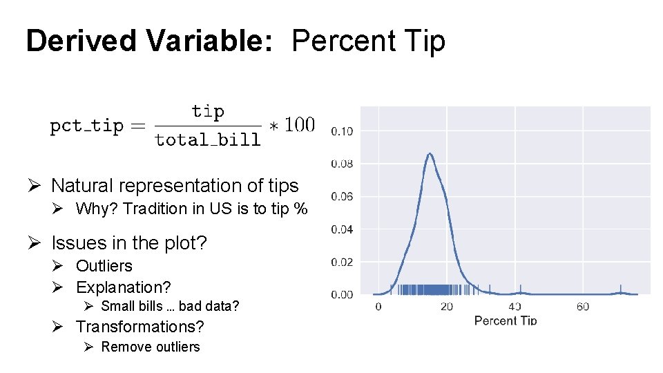
Derived Variable: Percent Tip Ø Natural representation of tips Ø Why? Tradition in US is to tip % Ø Issues in the plot? Ø Outliers Ø Explanation? Ø Small bills … bad data? Ø Transformations? Ø Remove outliers

Step 1: Define the Model START SIMPLE!!

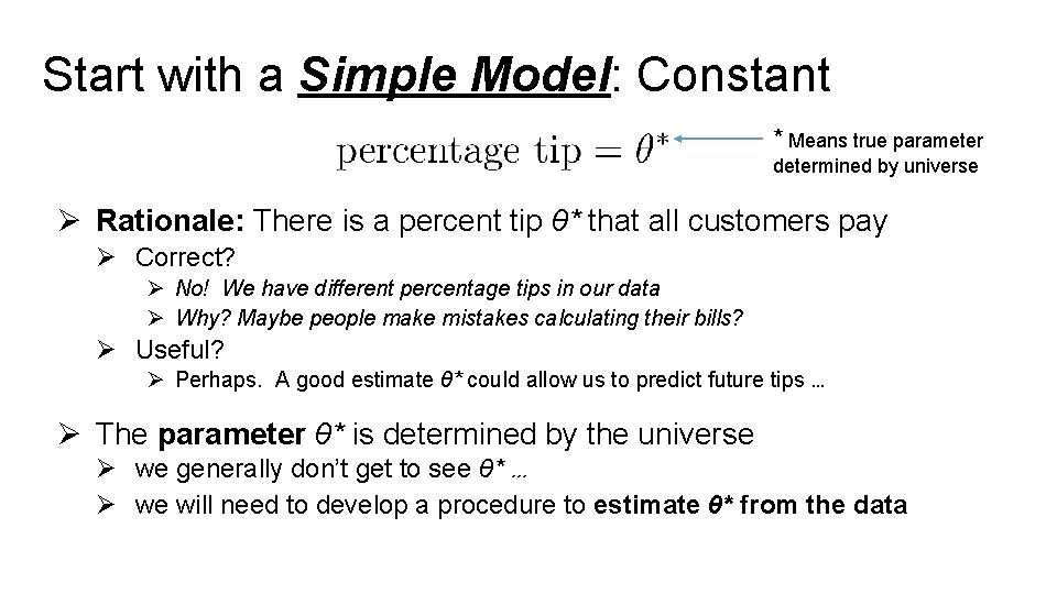
Start with a Simple Model: Constant * Means true parameter determined by universe Ø Rationale: There is a percent tip θ* that all customers pay Ø Correct? Ø No! We have different percentage tips in our data Ø Why? Maybe people make mistakes calculating their bills? Ø Useful? Ø Perhaps. A good estimate θ* could allow us to predict future tips … Ø The parameter θ* is determined by the universe Ø we generally don’t get to see θ* … Ø we will need to develop a procedure to estimate θ* from the data

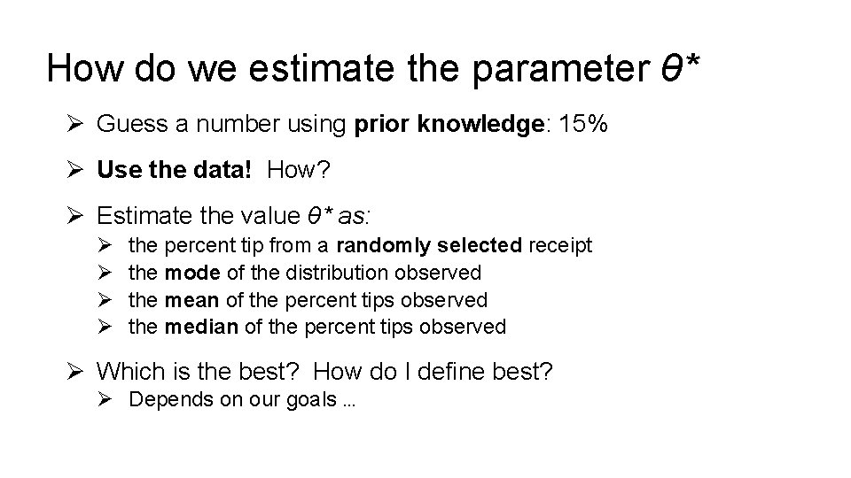
How do we estimate the parameter θ* Ø Guess a number using prior knowledge: 15% Ø Use the data! How? Ø Estimate the value θ* as: Ø Ø the percent tip from a randomly selected receipt the mode of the distribution observed the mean of the percent tips observed the median of the percent tips observed Ø Which is the best? How do I define best? Ø Depends on our goals …

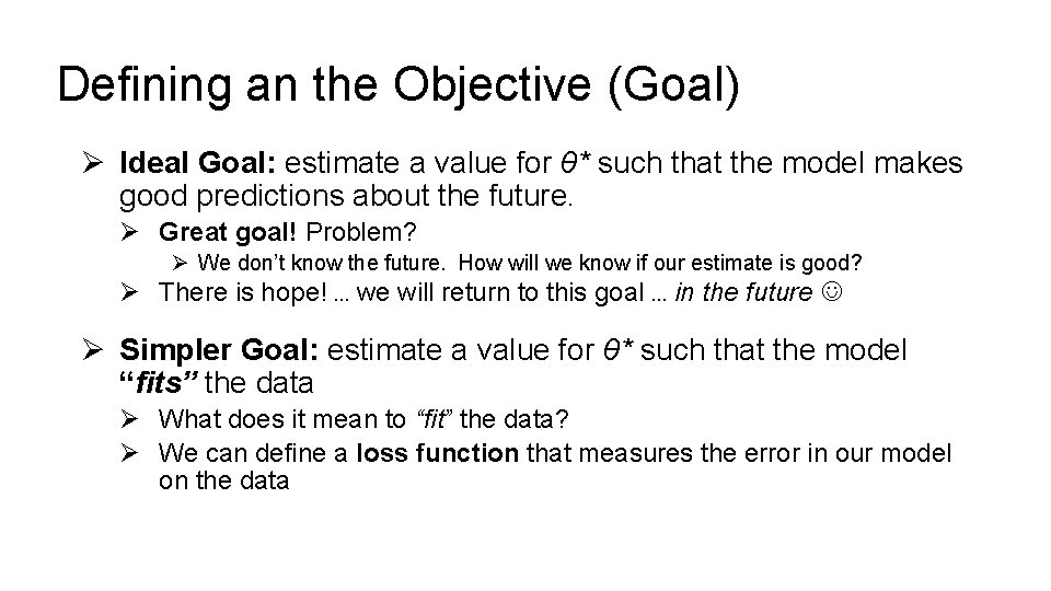
Defining an the Objective (Goal) Ø Ideal Goal: estimate a value for θ* such that the model makes good predictions about the future. Ø Great goal! Problem? Ø We don’t know the future. How will we know if our estimate is good? Ø There is hope! … we will return to this goal … in the future Ø Simpler Goal: estimate a value for θ* such that the model “fits” the data Ø What does it mean to “fit” the data? Ø We can define a loss function that measures the error in our model on the data

Step 2: Define the Loss “Take the Loss”

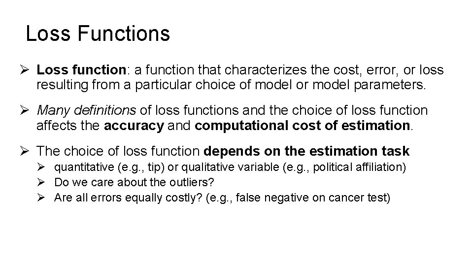
Loss Functions Ø Loss function: a function that characterizes the cost, error, or loss resulting from a particular choice of model or model parameters. Ø Many definitions of loss functions and the choice of loss function affects the accuracy and computational cost of estimation. Ø The choice of loss function depends on the estimation task Ø quantitative (e. g. , tip) or qualitative variable (e. g. , political affiliation) Ø Do we care about the outliers? Ø Are all errors equally costly? (e. g. , false negative on cancer test)

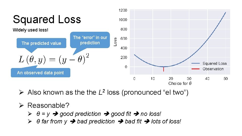
Squared Loss Widely used loss! The predicted value The “error” in our prediction An observed data point Ø Also known as the L 2 loss (pronounced “el two”) Ø Reasonable? Ø θ = y good prediction good fit no loss! Ø θ far from y bad prediction bad fit lots of loss!

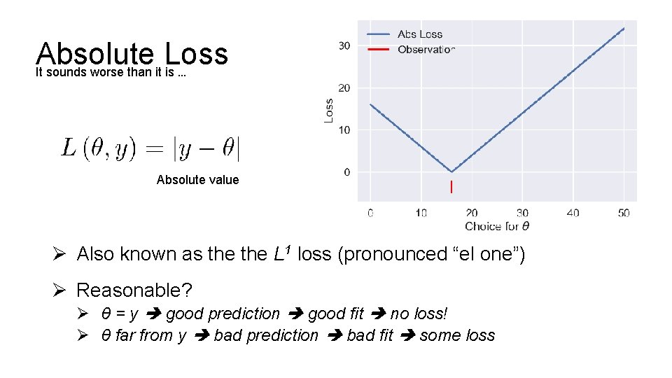
Absolute Loss It sounds worse than it is … Absolute value Ø Also known as the L 1 loss (pronounced “el one”) Ø Reasonable? Ø θ = y good prediction good fit no loss! Ø θ far from y bad prediction bad fit some loss

Can you think of another Loss Function?

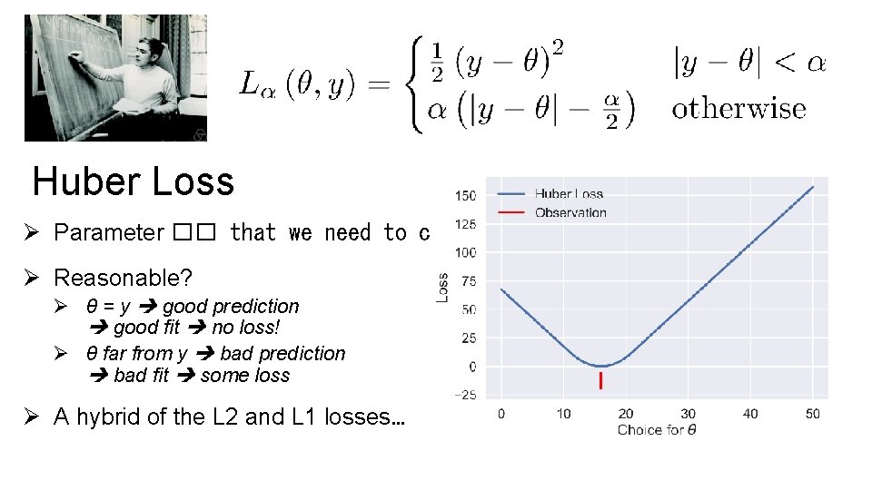
Huber Loss Ø Parameter �� that we need to choose. Ø Reasonable? Ø θ = y good prediction good fit no loss! Ø θ far from y bad prediction bad fit some loss Ø A hybrid of the L 2 and L 1 losses…

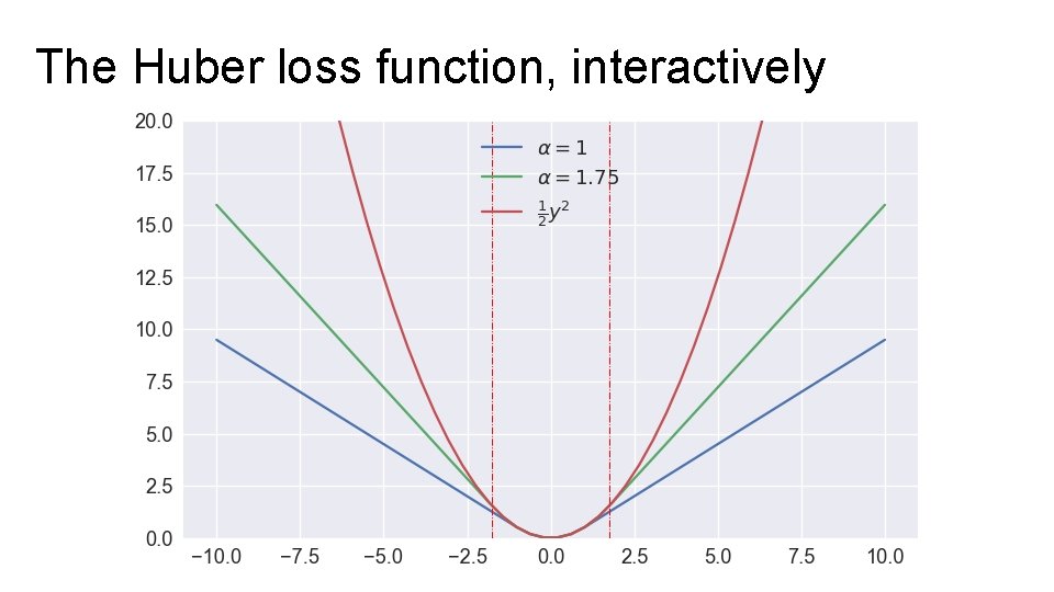
The Huber loss function, interactively

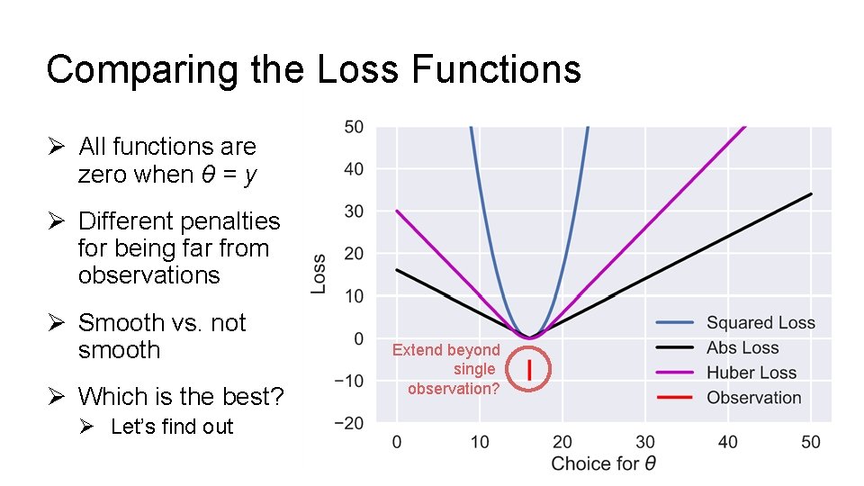
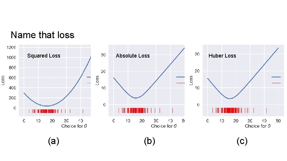
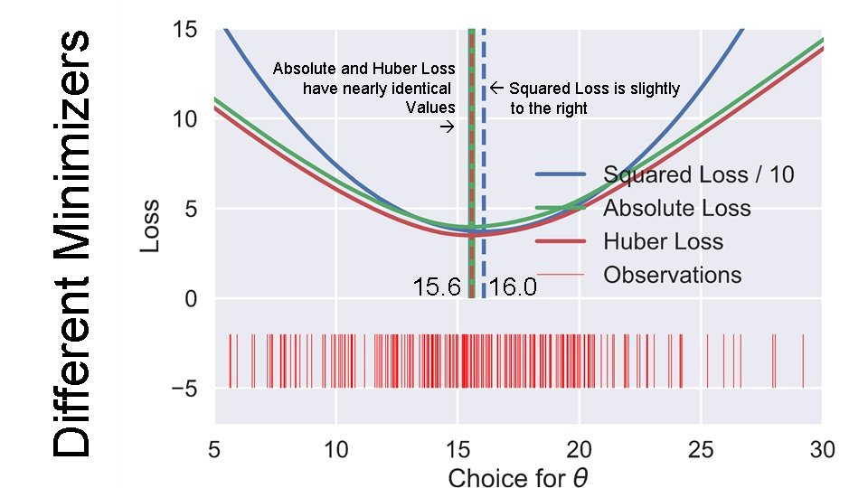
Comparing the Loss Functions Ø All functions are zero when θ = y Ø Different penalties for being far from observations Ø Smooth vs. not smooth Ø Which is the best? Ø Let’s find out Extend beyond single observation?

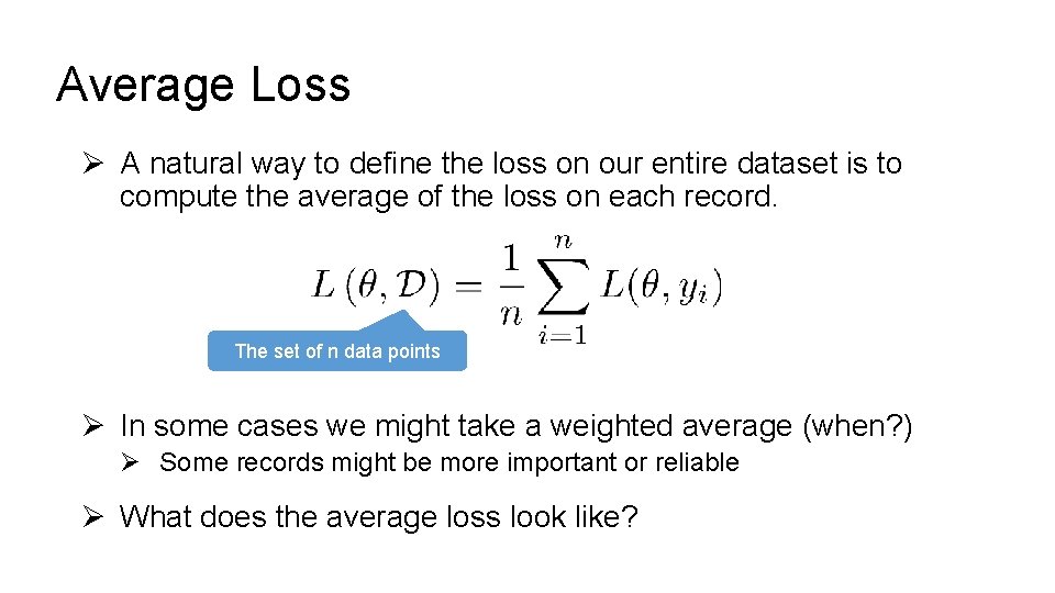
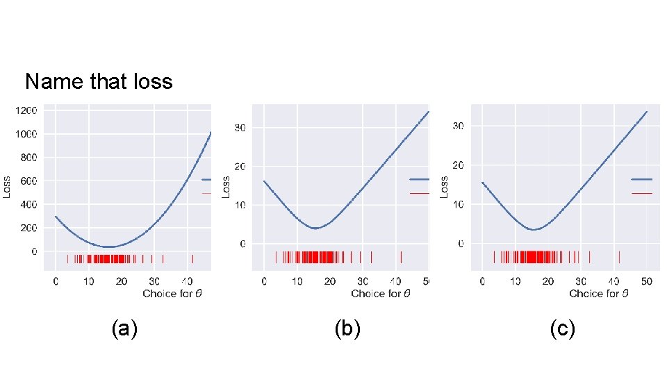
Average Loss Ø A natural way to define the loss on our entire dataset is to compute the average of the loss on each record. The set of n data points Ø In some cases we might take a weighted average (when? ) Ø Some records might be more important or reliable Ø What does the average loss look like?

Double Jeopardy Name that Loss!

Name that loss (a) (b) (c)

Name that loss Squared Loss (a) Absolute Loss (b) Huber Loss (c)

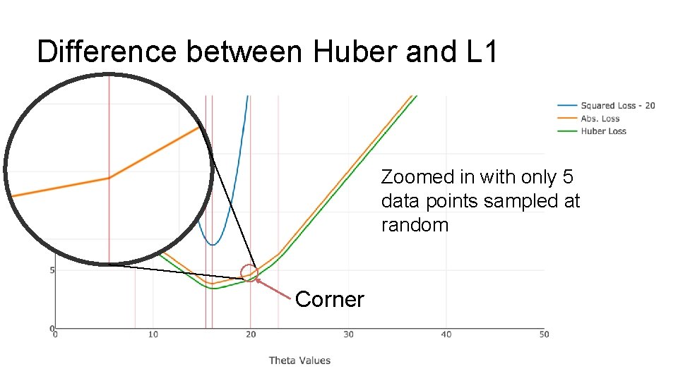
Difference between Huber and L 1 Zoomed in with only 5 data points sampled at random Corner

Different Minimizers Absolute and Huber Loss have nearly identical Values 15. 6 Squared Loss is slightly to the right 16. 0

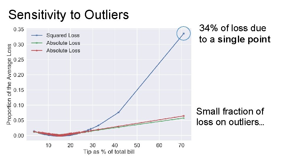
Sensitivity to Outliers 34% of loss due to a single point Small fraction of loss on outliers…

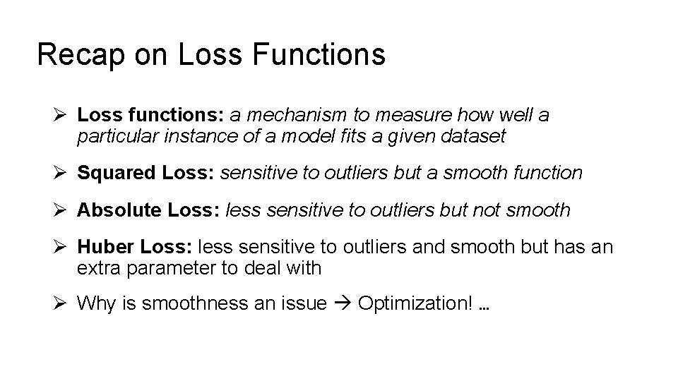
Recap on Loss Functions Ø Loss functions: a mechanism to measure how well a particular instance of a model fits a given dataset Ø Squared Loss: sensitive to outliers but a smooth function Ø Absolute Loss: less sensitive to outliers but not smooth Ø Huber Loss: less sensitive to outliers and smooth but has an extra parameter to deal with Ø Why is smoothness an issue Optimization! …

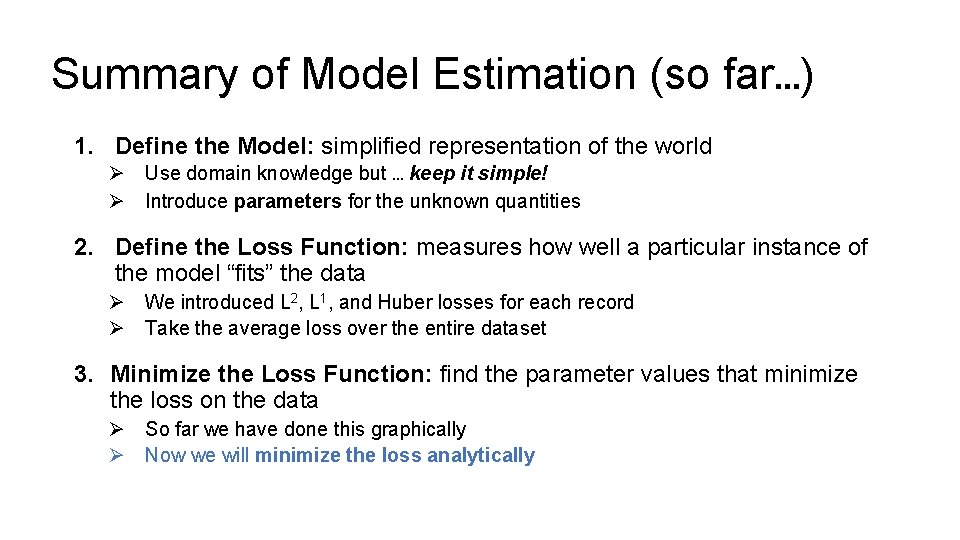
Summary of Model Estimation (so far…) 1. Define the Model: simplified representation of the world Ø Use domain knowledge but … keep it simple! Ø Introduce parameters for the unknown quantities 2. Define the Loss Function: measures how well a particular instance of the model “fits” the data Ø We introduced L 2, L 1, and Huber losses for each record Ø Take the average loss over the entire dataset 3. Minimize the Loss Function: find the parameter values that minimize the loss on the data Ø So far we have done this graphically Ø Now we will minimize the loss analytically

Step 3: Minimize the Loss

A Brief Review of Calculus

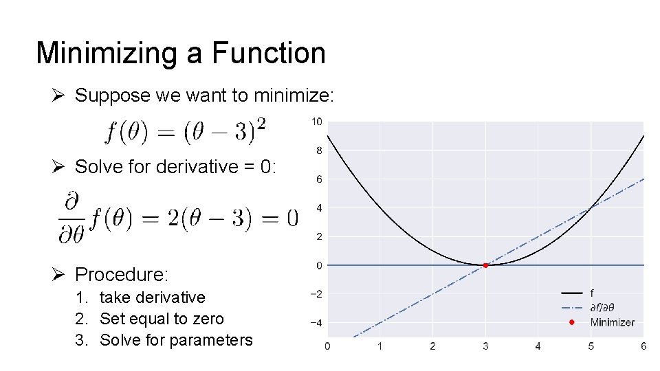
Minimizing a Function Ø Suppose we want to minimize: Ø Solve for derivative = 0: Ø Procedure: 1. take derivative 2. Set equal to zero 3. Solve for parameters

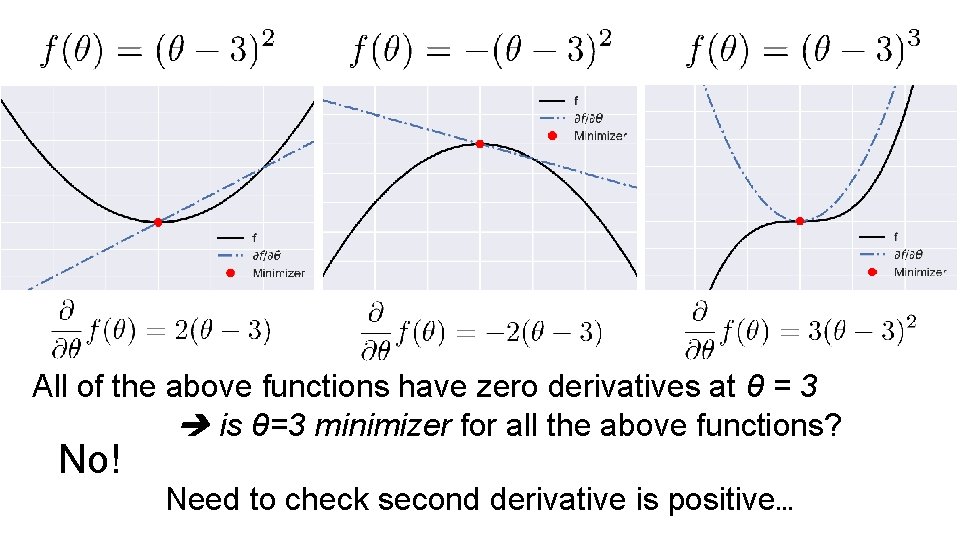
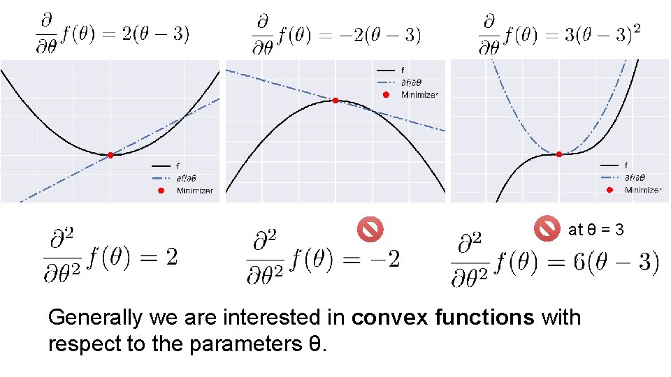
All of the above functions have zero derivatives at θ = 3 is θ=3 minimizer for all the above functions? No! Need to check second derivative is positive…

at θ = 3 Generally we are interested in convex functions with respect to the parameters θ.

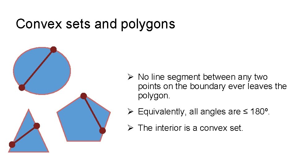
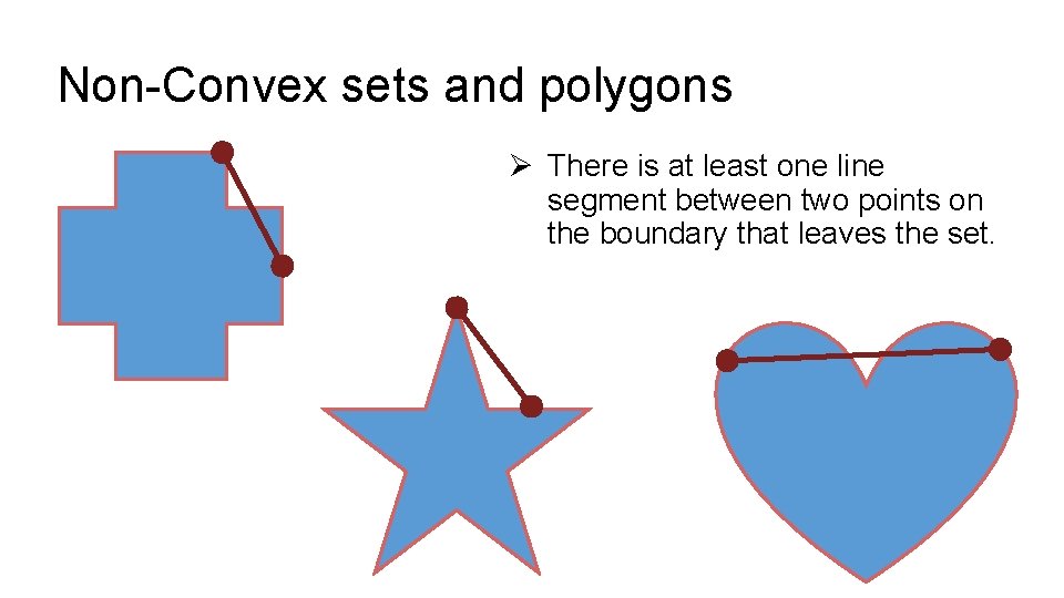
Convex sets and polygons Ø No line segment between any two points on the boundary ever leaves the polygon. Ø Equivalently, all angles are ≤ 180º. Ø The interior is a convex set.

Non-Convex sets and polygons Ø There is at least one line segment between two points on the boundary that leaves the set.

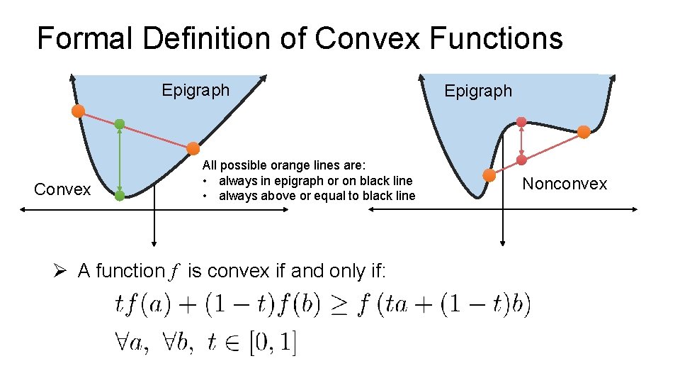
Formal Definition of Convex Functions Epigraph Convex All possible orange lines are: • always in epigraph or on black line • always above or equal to black line Ø A function f is convex if and only if: Epigraph Nonconvex

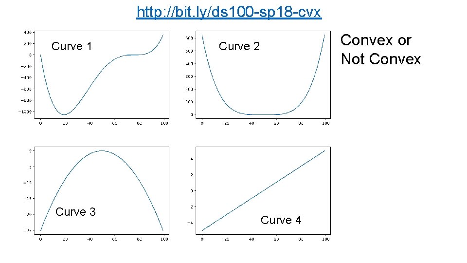
http: //bit. ly/ds 100 -sp 18 -cvx Curve 1 Curve 3 Convex or Not Convex Curve 2 Curve 4

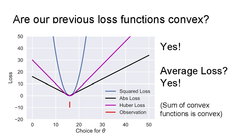
Are our previous loss functions convex? Yes! Average Loss? Yes! (Sum of convex functions is convex)

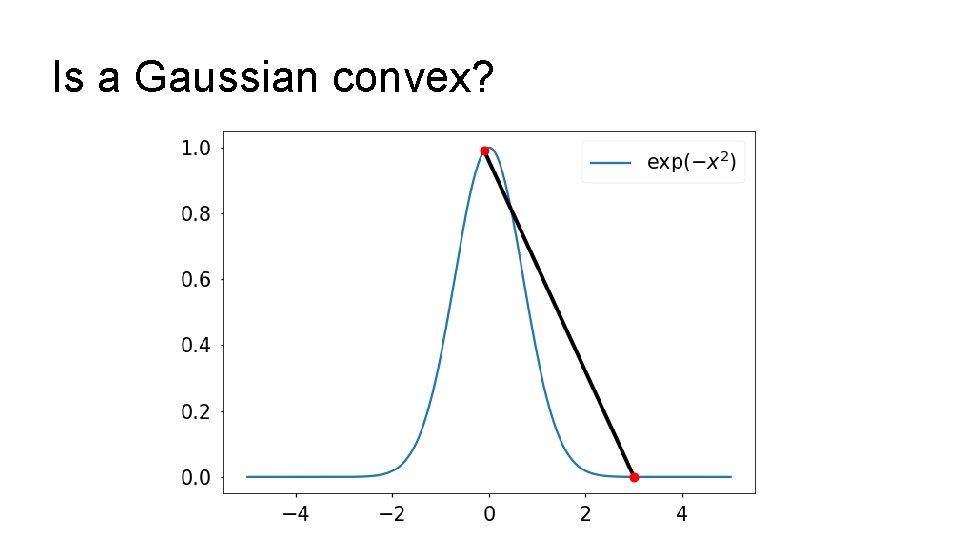
Is a Gaussian convex?

Minimizing the Average Squared Loss

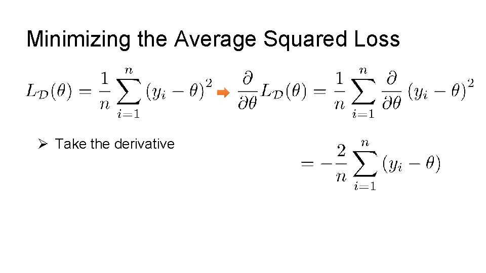
Minimizing the Average Squared Loss Ø Take the derivative

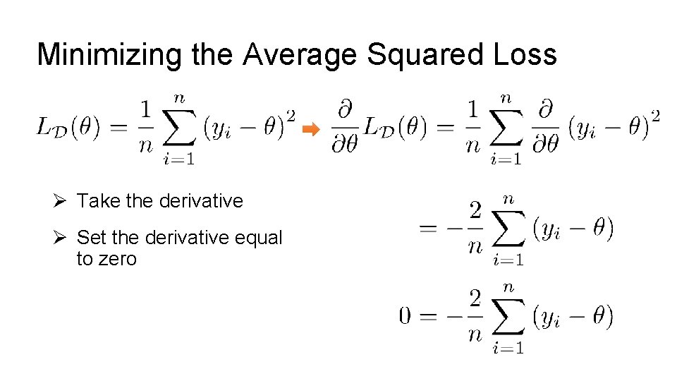
Minimizing the Average Squared Loss Ø Take the derivative Ø Set the derivative equal to zero

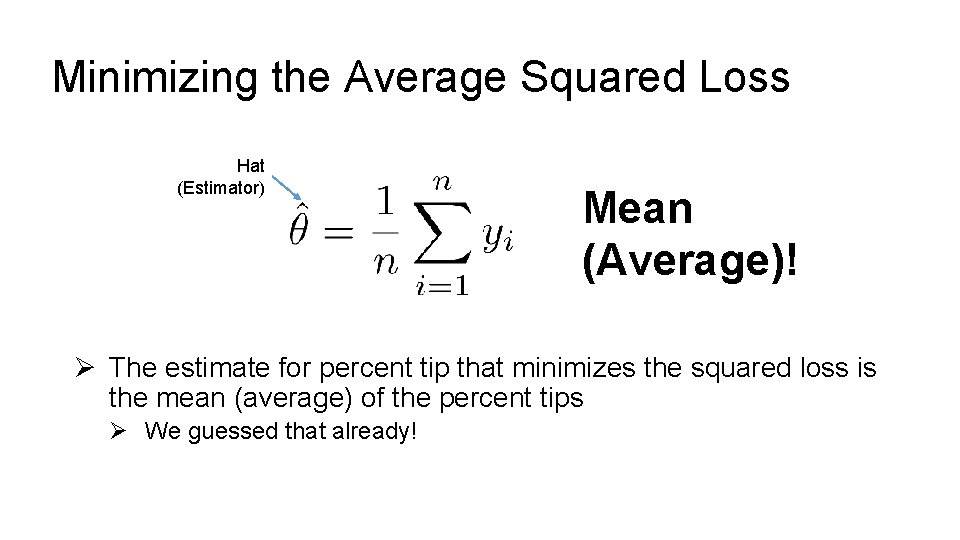
Minimizing the Average Squared Loss Ø Take the derivative Ø Set the derivative equal to zero Ø Solve for parameters Hat (Estimator)

Minimizing the Average Squared Loss Hat (Estimator) Mean (Average)! Ø The estimate for percent tip that minimizes the squared loss is the mean (average) of the percent tips Ø We guessed that already!

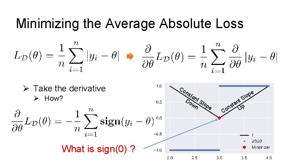
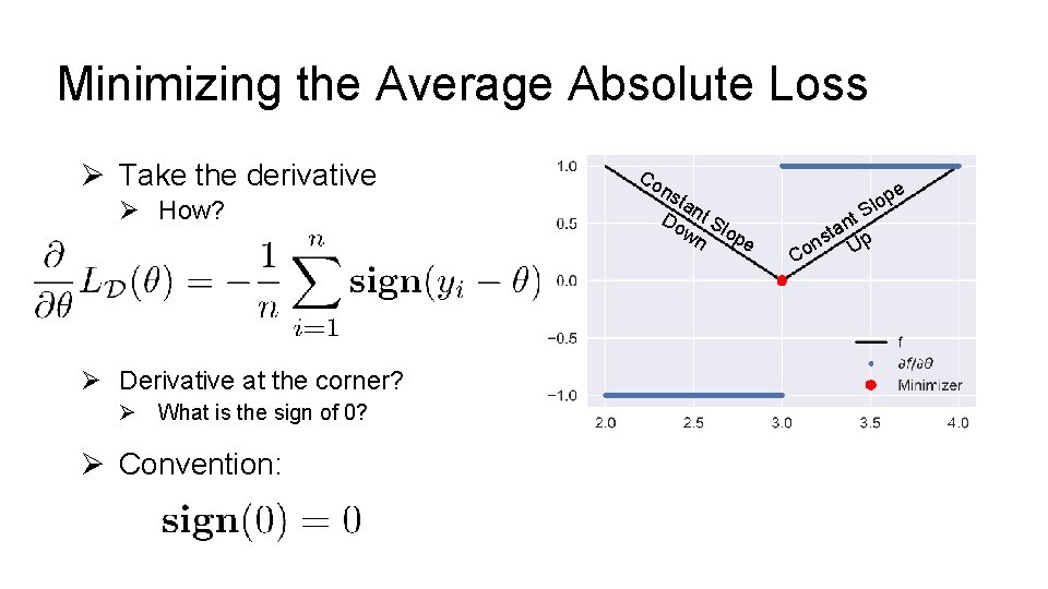
Minimizing the Average Absolute Loss Ø Take the derivative Ø How? What is sign(0) ? Co n sta Do nt S wn lop e e p o l S C t n a st p on U

Minimizing the Average Absolute Loss Ø Take the derivative Ø How? Ø Derivative at the corner? Ø What is the sign of 0? Ø Convention: Co n sta Do nt S wn lop e e p o l S C nt a t s p on U

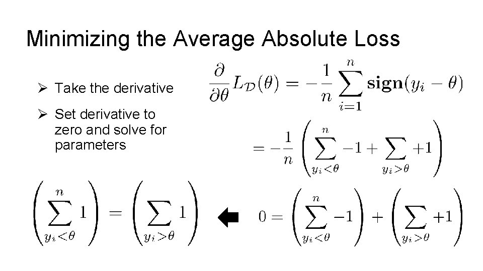
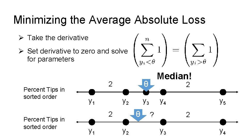
Minimizing the Average Absolute Loss Ø Take the derivative Ø Set derivative to zero and solve for parameters

Minimizing the Average Absolute Loss Ø Take the derivative Ø Set derivative to zero and solve for parameters Percent Tips in sorted order θ 2 y 1 y 2 2 y 3 θ 2 y 1 Median! y 4 ? y 5 2 y 3 y 4

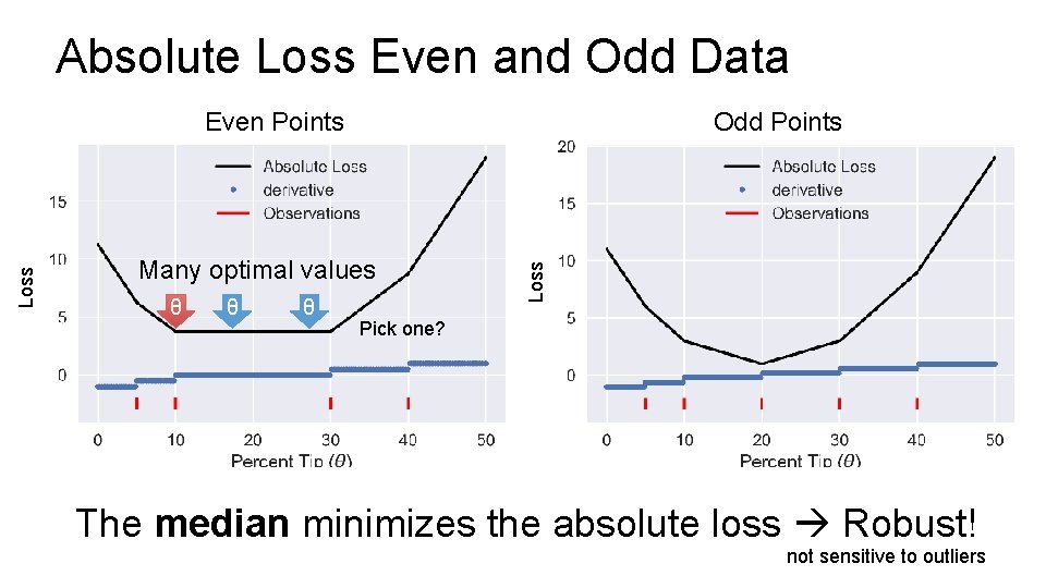
Absolute Loss Even and Odd Data Odd Points Many optimal values θ θ θ Loss Even Points Pick one? The median minimizes the absolute loss Robust! not sensitive to outliers

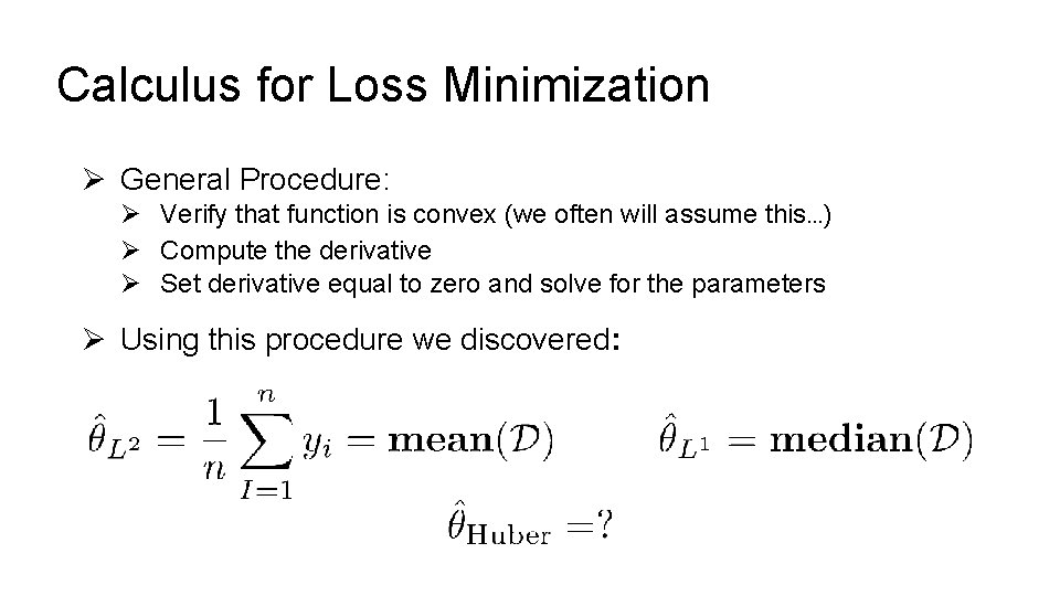
Calculus for Loss Minimization Ø General Procedure: Ø Verify that function is convex (we often will assume this…) Ø Compute the derivative Ø Set derivative equal to zero and solve for the parameters Ø Using this procedure we discovered: