Data Processing Why Preprocess the data Todays realworld

Data Processing

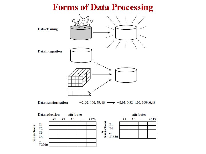
Why Preprocess the data? § Today’s real-world databases are highly susceptible to noisy, missing, and inconsistent data due to their typically huge size (often several gigabytes or more) and their likely origin from multiple, heterogeneous sources. § Low-quality data will lead to low-quality mining results. § There a number of data preprocessing techniques. Data cleaning, Data integration, Data transformations, Data reduction § These techniques are not mutually exclusive; they may work together.

Why Preprocess the data? Incomplete data can occur for a number of reasons. § Attributes of interest may not always be available, such as customer information for sales transaction data. § Other data may not be included simply because it was not considered important at the time of entry. § Relevant data may not be recorded due to a misunderstanding, or because of equipment malfunctions.

Why Preprocess the data? § There are many possible reasons for noisy data (having incorrect attribute values). § The data collection instruments used may be faulty. § There may have been human or computer errors occurring at data entry. § Errors in data transmission can also occur. § There may be technology limitations, such as limited buffer size for coordinating synchronized data transfer and consumption.

Forms of Data Processing

Data Cleaning § Real-world data tend to be incomplete, noisy, and inconsistent. § Data cleaning routines attempt to fill in missing values, smooth out noise while identifying outliers, and correct inconsistencies in the data. Methods for Missing Values Ignore the tuple: § This is usually done when the class label is missing (assuming the mining task involves classification). § This method is not very effective, unless the tuple contains several attributes with missing values. Fill in the missing value manually: § In general, this approach is time-consuming and may not be feasible given a large data set with many missing values.

Data Cleaning Use a global constant to fill in the missing value: § Replace all missing attribute values by the same constant, such as a label like “Unknown” or ∞. § If missing values are replaced by, say, “Unknown, ” then the mining program may mistakenly think that they form an interesting concept, since they all have a value in common—that of “Unknown. ” Hence, although this method is simple, it is not foolproof. Use the attribute mean to fill in the missing value: § For example, suppose that the average income of All. Electronics customers is $56, 000. Use this value to replace the missing value for income. Use the attribute mean for all samples belonging to the same class : § For example, if classifying customers according to credit risk, replace the missing value with the average income value for customers in the same credit risk category as that of the given tuple.

Data Cleaning Use the most probable value to fill in the missing value: § This may be determined with regression, inference-based tools using a Bayesian formalism, or decision tree induction. § For example, using the other customer attributes in your data set, you may construct a decision tree to predict the missing values for income. § The filled-in value using above methods may not be correct. § however, Use the most probable value to fill in the missing value is a popular strategy. In comparison to the other methods, it uses the most information from the present data to predict missing values. § It is important to note that, in some cases, a missing value may not imply an error in the data! For example, when applying for a credit card, candidates may be asked to supply their driver’s license number. Candidates who do not have a driver’s license may naturally leave this field blank.

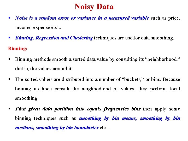
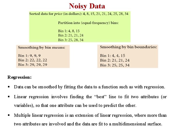
Noisy Data § Noise is a random error or variance in a measured variable such as price, income, expense etc. . . § Binning, Regression and Clustering techniques are use for data smoothing. Binning: § Binning methods smooth a sorted data value by consulting its “neighborhood, ” that is, the values around it. § The sorted values are distributed into a number of “buckets, ” or bins. Because binning methods consult the neighborhood of values, they perform local smoothing § First given data partition into equals frequencies bins then apply some binning techniques such as smoothing by bin means, smoothing by bin medians, smoothing by bin boundaries etc…

Noisy Data Regression: § Data can be smoothed by fitting the data to a function such as with regression. § Linear regression involves finding the “best” line to fit two attributes (or variables), so that one attribute can be used to predict the other. § Multiple linear regression is an extension of linear regression, where more than two attributes are involved and the data are fit to a multidimensional surface.

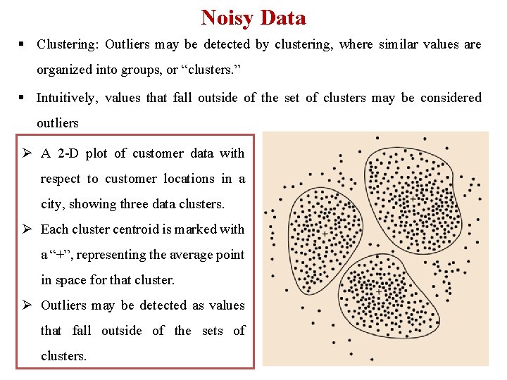
Noisy Data § Clustering: Outliers may be detected by clustering, where similar values are organized into groups, or “clusters. ” § Intuitively, values that fall outside of the set of clusters may be considered outliers Ø A 2 -D plot of customer data with respect to customer locations in a city, showing three data clusters. Ø Each cluster centroid is marked with a “+”, representing the average point in space for that cluster. Ø Outliers may be detected as values that fall outside of the sets of clusters.

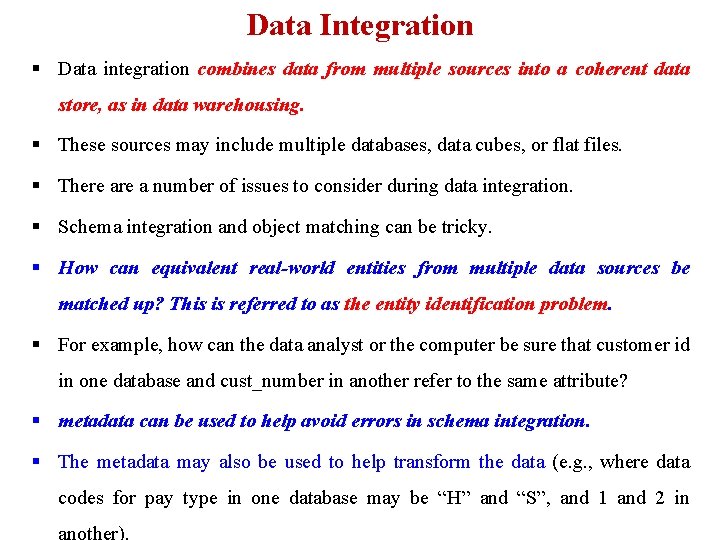
Data Integration § Data integration combines data from multiple sources into a coherent data store, as in data warehousing. § These sources may include multiple databases, data cubes, or flat files. § There a number of issues to consider during data integration. § Schema integration and object matching can be tricky. § How can equivalent real-world entities from multiple data sources be matched up? This is referred to as the entity identification problem. § For example, how can the data analyst or the computer be sure that customer id in one database and cust_number in another refer to the same attribute? § metadata can be used to help avoid errors in schema integration. § The metadata may also be used to help transform the data (e. g. , where data codes for pay type in one database may be “H” and “S”, and 1 and 2 in

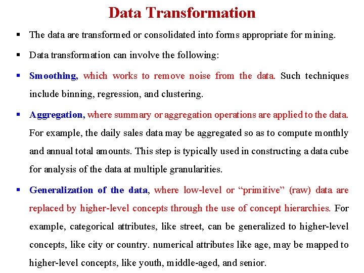
Data Transformation § The data are transformed or consolidated into forms appropriate for mining. § Data transformation can involve the following: § Smoothing, which works to remove noise from the data. Such techniques include binning, regression, and clustering. § Aggregation, where summary or aggregation operations are applied to the data. For example, the daily sales data may be aggregated so as to compute monthly and annual total amounts. This step is typically used in constructing a data cube for analysis of the data at multiple granularities. § Generalization of the data, where low-level or “primitive” (raw) data are replaced by higher-level concepts through the use of concept hierarchies. For example, categorical attributes, like street, can be generalized to higher-level concepts, like city or country. numerical attributes like age, may be mapped to higher-level concepts, like youth, middle-aged, and senior.

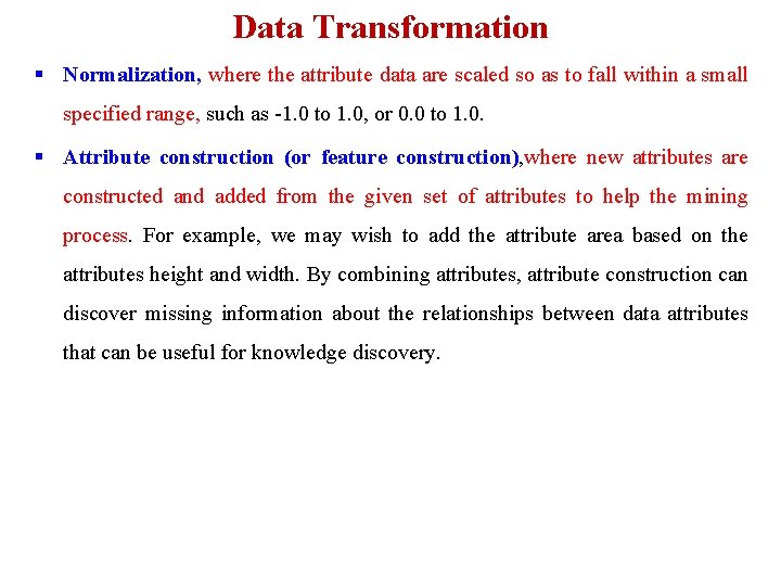
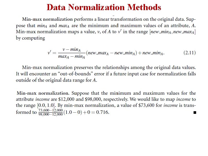
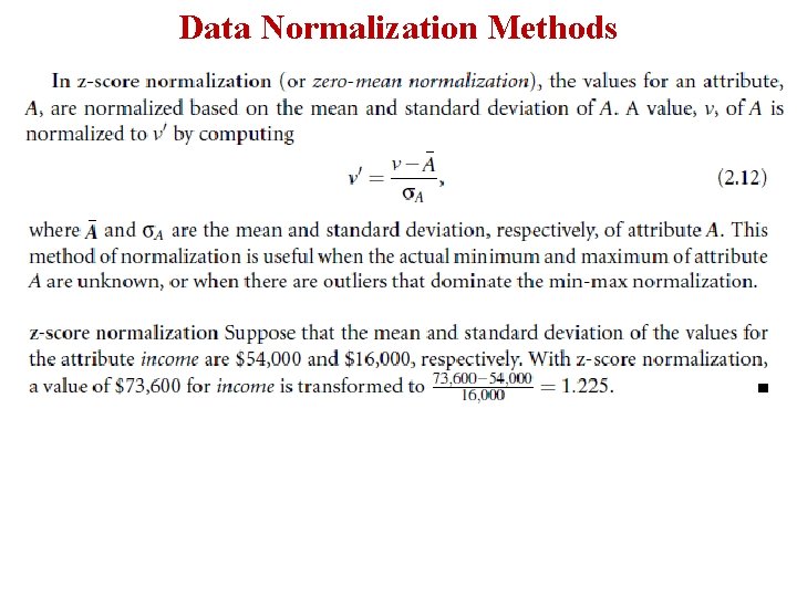
Data Transformation § Normalization, where the attribute data are scaled so as to fall within a small specified range, such as -1. 0 to 1. 0, or 0. 0 to 1. 0. § Attribute construction (or feature construction), where new attributes are constructed and added from the given set of attributes to help the mining process. For example, we may wish to add the attribute area based on the attributes height and width. By combining attributes, attribute construction can discover missing information about the relationships between data attributes that can be useful for knowledge discovery.

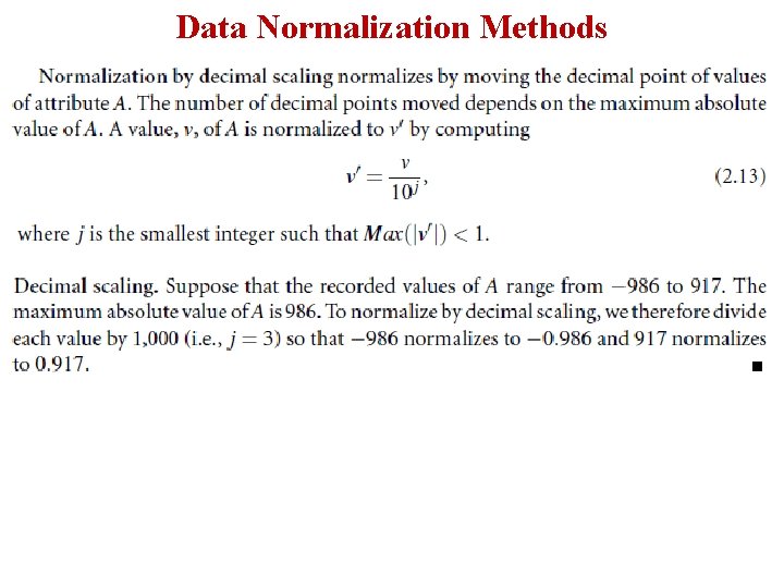
Data Normalization Methods

Data Normalization Methods

Data Normalization Methods

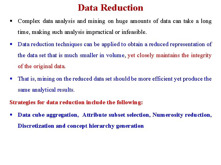
Data Reduction § Complex data analysis and mining on huge amounts of data can take a long time, making such analysis impractical or infeasible. § Data reduction techniques can be applied to obtain a reduced representation of the data set that is much smaller in volume, yet closely maintains the integrity of the original data. § That is, mining on the reduced data set should be more efficient yet produce the same analytical results. Strategies for data reduction include the following: § Data cube aggregation, Attribute subset selection, Numerosity reduction, Discretization and concept hierarchy generation

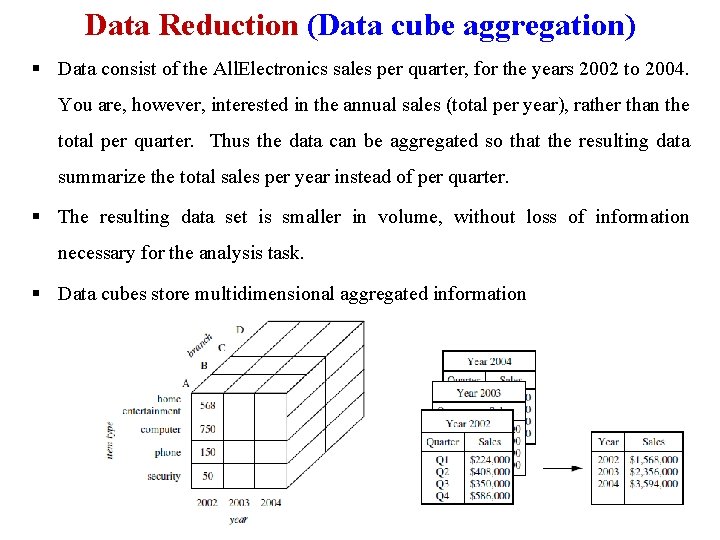
Data Reduction (Data cube aggregation) § Data consist of the All. Electronics sales per quarter, for the years 2002 to 2004. You are, however, interested in the annual sales (total per year), rather than the total per quarter. Thus the data can be aggregated so that the resulting data summarize the total sales per year instead of per quarter. § The resulting data set is smaller in volume, without loss of information necessary for the analysis task. § Data cubes store multidimensional aggregated information

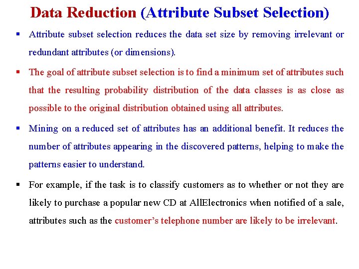
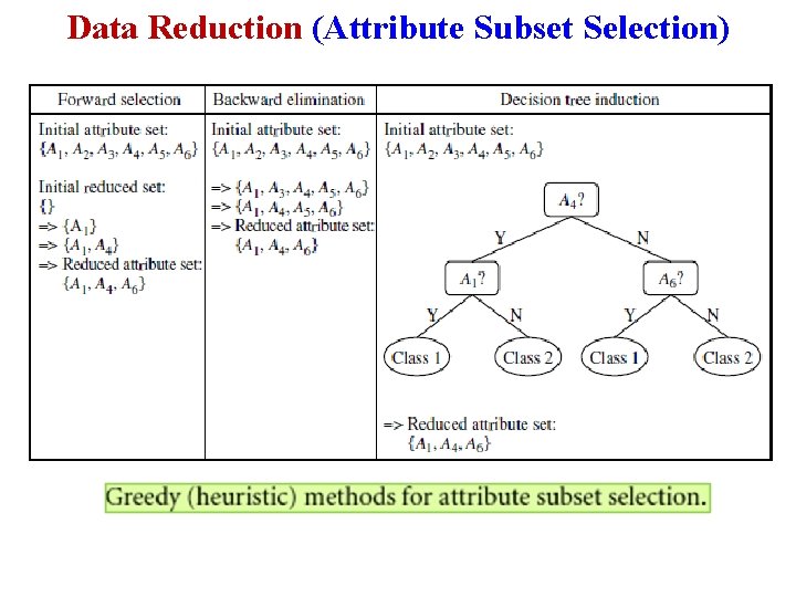
Data Reduction (Attribute Subset Selection) § Attribute subset selection reduces the data set size by removing irrelevant or redundant attributes (or dimensions). § The goal of attribute subset selection is to find a minimum set of attributes such that the resulting probability distribution of the data classes is as close as possible to the original distribution obtained using all attributes. § Mining on a reduced set of attributes has an additional benefit. It reduces the number of attributes appearing in the discovered patterns, helping to make the patterns easier to understand. § For example, if the task is to classify customers as to whether or not they are likely to purchase a popular new CD at All. Electronics when notified of a sale, attributes such as the customer’s telephone number are likely to be irrelevant.

Data Reduction (Attribute Subset Selection) § Although it may be possible for a domain expert to pick out some of the useful attributes, this can be a difficult and time-consuming task, especially when the behavior of the data is not well known. § Leaving out relevant attributes or keeping irrelevant attributes may be detrimental, causing confusion for the mining algorithm employed. This can result in discovered patterns of poor quality.

Data Reduction (Attribute Subset Selection)

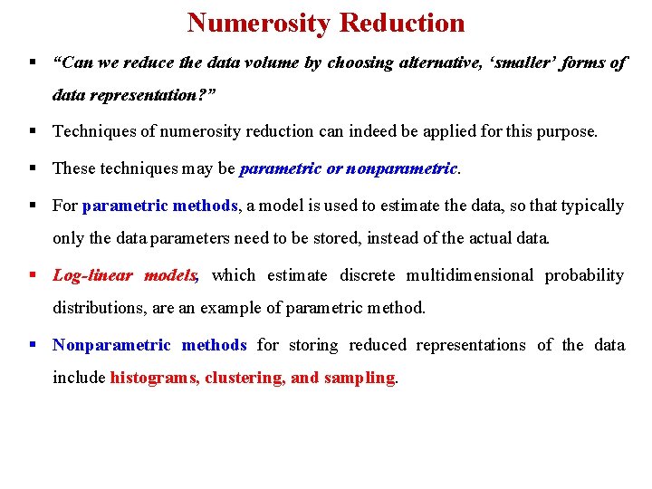
Numerosity Reduction § “Can we reduce the data volume by choosing alternative, ‘smaller’ forms of data representation? ” § Techniques of numerosity reduction can indeed be applied for this purpose. § These techniques may be parametric or nonparametric. § For parametric methods, a model is used to estimate the data, so that typically only the data parameters need to be stored, instead of the actual data. § Log-linear models, which estimate discrete multidimensional probability distributions, are an example of parametric method. § Nonparametric methods for storing reduced representations of the data include histograms, clustering, and sampling.

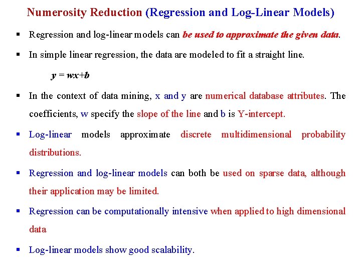
Numerosity Reduction (Regression and Log-Linear Models) § Regression and log-linear models can be used to approximate the given data. § In simple linear regression, the data are modeled to fit a straight line. y = wx+b § In the context of data mining, x and y are numerical database attributes. The coefficients, w specify the slope of the line and b is Y-intercept. § Log-linear models approximate discrete multidimensional probability distributions. § Regression and log-linear models can both be used on sparse data, although their application may be limited. § Regression can be computationally intensive when applied to high dimensional data § Log-linear models show good scalability.

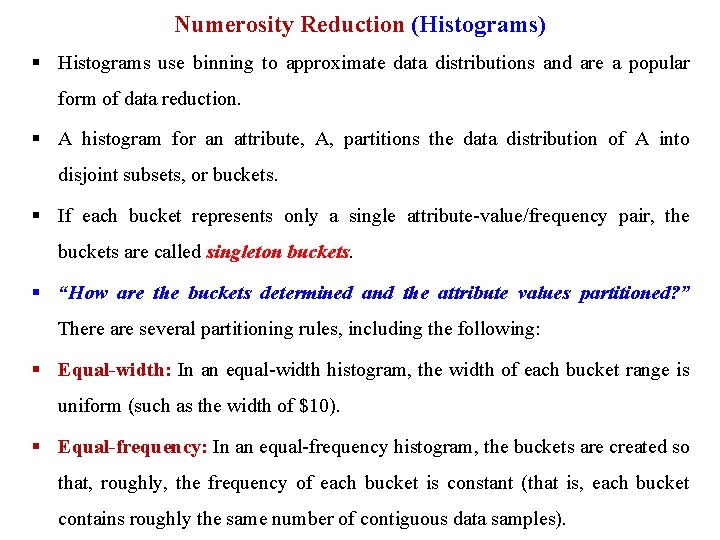
Numerosity Reduction (Histograms) § Histograms use binning to approximate data distributions and are a popular form of data reduction. § A histogram for an attribute, A, partitions the data distribution of A into disjoint subsets, or buckets. § If each bucket represents only a single attribute-value/frequency pair, the buckets are called singleton buckets. § “How are the buckets determined and the attribute values partitioned? ” There are several partitioning rules, including the following: § Equal-width: In an equal-width histogram, the width of each bucket range is uniform (such as the width of $10). § Equal-frequency: In an equal-frequency histogram, the buckets are created so that, roughly, the frequency of each bucket is constant (that is, each bucket contains roughly the same number of contiguous data samples).

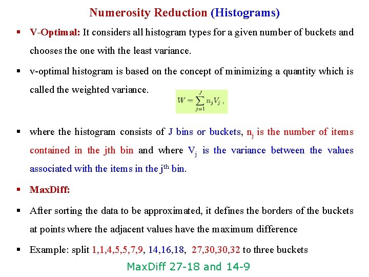
Numerosity Reduction (Histograms) § V-Optimal: It considers all histogram types for a given number of buckets and chooses the one with the least variance. § v-optimal histogram is based on the concept of minimizing a quantity which is called the weighted variance. § where the histogram consists of J bins or buckets, nj is the number of items contained in the jth bin and where Vj is the variance between the values associated with the items in the jth bin. § Max. Diff: § After sorting the data to be approximated, it defines the borders of the buckets at points where the adjacent values have the maximum difference § Example: split 1, 1, 4, 5, 5, 7, 9, 14, 16, 18, 27, 30, 32 to three buckets Max. Diff 27 -18 and 14 -9

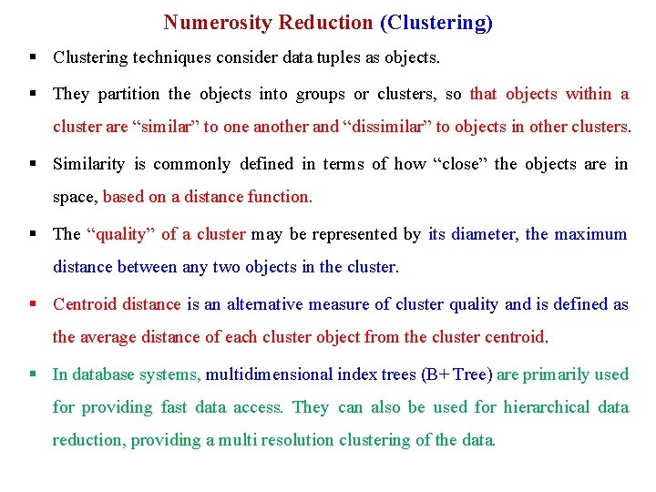
Numerosity Reduction (Clustering) § Clustering techniques consider data tuples as objects. § They partition the objects into groups or clusters, so that objects within a cluster are “similar” to one another and “dissimilar” to objects in other clusters. § Similarity is commonly defined in terms of how “close” the objects are in space, based on a distance function. § The “quality” of a cluster may be represented by its diameter, the maximum distance between any two objects in the cluster. § Centroid distance is an alternative measure of cluster quality and is defined as the average distance of each cluster object from the cluster centroid. § In database systems, multidimensional index trees (B+ Tree) are primarily used for providing fast data access. They can also be used for hierarchical data reduction, providing a multi resolution clustering of the data.

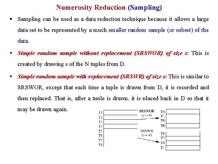
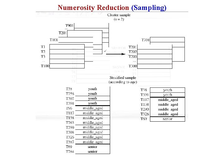
Numerosity Reduction (Sampling) § Sampling can be used as a data reduction technique because it allows a large data set to be represented by a much smaller random sample (or subset) of the data. § Simple random sample without replacement (SRSWOR) of size s: This is created by drawing s of the N tuples from D. § Simple random sample with replacement (SRSWR) of size s: This is similar to SRSWOR, except that each time a tuple is drawn from D, it is recorded and then replaced. That is, after a tuple is drawn, it is placed back in D so that it may be drawn again.

Numerosity Reduction (Sampling)

Data Discretization § Data discretization techniques can be used to reduce the number of values for a given continuous attribute by dividing the range of the attribute into intervals. § Interval labels can then be used to replace actual data values. § Replacing numerous values of a continuous attribute by a small number of interval labels thereby reduces and simplifies the original data. § Data Discretization leads to a concise, easy-to-use, knowledge-level representation of mining results. § Discretization techniques can be categorized based on how the discretization is performed, such as whether it uses class information or which direction it proceeds (i. e. , top-down vs. bottom-up). § If the discretization process uses class information, then we say it is supervised discretization. Otherwise, it is unsupervised.

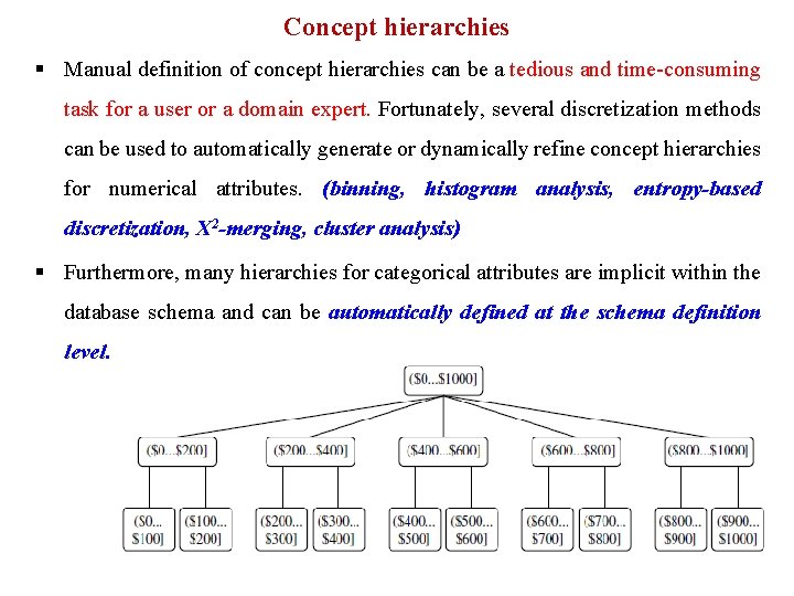
Data Discretization § If the process starts by first finding one or a few points (called split points or cut points) to split the entire attribute range, and then repeats this recursively on the resulting intervals, it is called top-down discretization or splitting. § This contrasts with bottom-up discretization or merging, which starts by considering all of the continuous values as potential split-points, removes some by merging neighborhood values to form intervals, and then recursively applies this process to the resulting intervals. § Discretization can be performed recursively on an attribute to provide a hierarchical or multi resolution partitioning of the attribute values, known as a concept hierarchy. § Concept hierarchies are useful for mining at multiple levels of abstraction.

Concept hierarchies § A concept hierarchy for a given numerical attribute defines a discretization of the attribute. § Concept hierarchies can be used to reduce the data by collecting and replacing low-level concepts (such as numerical values for the attribute age) with higherlevel concepts (such as youth, middle-aged, or senior). § the generalized data may be more meaningful and easier to interpret. § This contributes to a consistent representation of data mining results among multiple mining tasks, which is a common requirement. § In addition, mining on a reduced data set requires fewer input/output operations and is more efficient than mining on a larger, ungeneralized data set. § Because of these benefits, discretization techniques and concept hierarchies are typically applied before data mining as a preprocessing step, rather than during mining.

Concept hierarchies § Manual definition of concept hierarchies can be a tedious and time-consuming task for a user or a domain expert. Fortunately, several discretization methods can be used to automatically generate or dynamically refine concept hierarchies for numerical attributes. (binning, histogram analysis, entropy-based discretization, X 2 -merging, cluster analysis) § Furthermore, many hierarchies for categorical attributes are implicit within the database schema and can be automatically defined at the schema definition level.

Thank You