Data Modeling Database Design Concepts 12262021 Jahangir Alam

Data Modeling & Database Design Concepts 12/26/2021 Jahangir Alam 1

Data Models • We know that a schema is written using a data definition language. In fact it is written in the data definition language of a particular DBMS. • Unfortunately, this type of language is too low level to describe the data requirements of an organization in a way that is readily understandable by a variety of users. What we require is a higher level description of the schema, i. e. a data model. • A model is a representation of real world objects and their associations. A data model in fact represents the organization itself. • It should provide the basic concepts and notations that will allow the database designers and end users unambiguously and accurately to communicate their understanding of the organizational data. A data model can be thought of as comprising the following three components: 12/26/2021 Jahangir Alam 2

• A Structural Part, consisting a set of rules according to which database can be constructed. • A Manipulative Part, defining the types of operations that are allowed on the data • A set of Integrity Rules which ensures that the data is accurate. • The purpose of a data model is to represent the data and to make the data understandable. If it does this then it can be easily used to design a database. • There have been many data models proposed in literature and we can categorize them according to the types of concepts they use to describe the database structure. • High Level or Conceptual Data Models provide concepts that are close to the way many users perceive data, whereas Low. Level or Physical Data Models provide concepts that describe the details of how data is stored in the memory of the computer. 12/26/2021 Jahangir Alam 3

• Concepts provided by low-level data models are generally meant for computer specialists, not for typical end users. • Between these two extremes is a class of Representational (or implementation or traditional) Data Models, which provide concepts that may be understood by end users but they are not too far removed from the way data is organized within the memory of computer. • Representational data models hide some (not all) details of data storage but can be implemented on a computer system in a direct way. • Conceptual Data Models use concepts such as entities, attributes and relationships. (We shall discuss ER Model in detail). • Representational Data Models are the models used most frequently in traditional commercial DBMSs, and they include the most widely used relational data model as well as the so-called legacy data models – the Network and Hierarchical Data Models. 12/26/2021 Jahangir Alam 4

• Representational Data Models represent data by using record structures ( a characteristics close to physical data models) and hence are referred to as Record Based Data Models. • We can regard Object Data Models as a new family of high level implementation data models that are closer to the conceptual data models. Object Data Models are frequently utilized as high level conceptual data models, particularly in the Software Engineering Domain. • In practice Conceptual Data Models are used to derive the highest level abstraction of the database and the model thus obtained is converted to representational data model that can be directly implemented on a computer (i. e. that can be utilized to create conceptual and external schemas). • In the next few portions of this lecture we shall discuss Conceptual and Representational Data Models at length and shall briefly discuss Object Data Models. • We shall begin our discussion with the most essential topic of data associations. 12/26/2021 Jahangir Alam 5

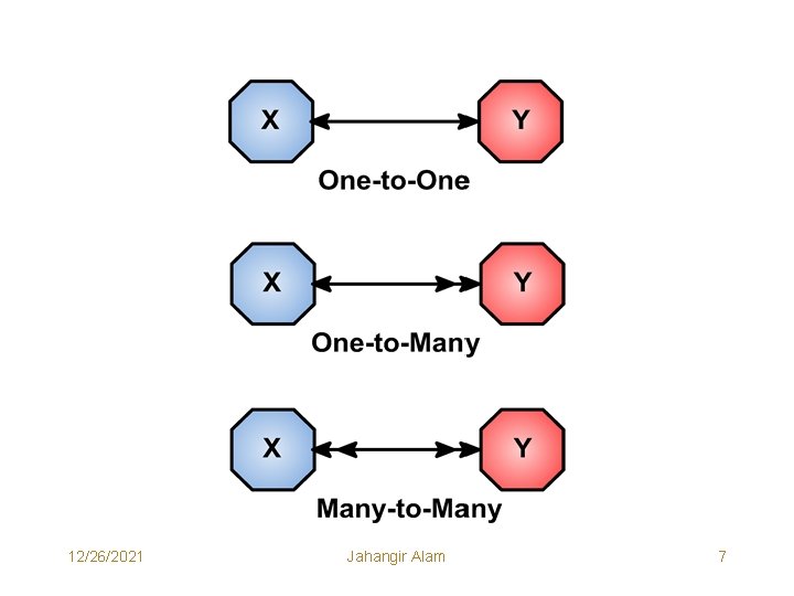
Data Associations • Data Associations means relationship between various data items (Entities and Attributes). Data Modeling in fact is used to represent the entities of Interest and their relationships in the database. • Entities specify distinct real world items in an application. Basically they are nouns or in other words anything of the interest of the organization. • Attributes are nothing but the properties of Entities. • When a large amount of data is stored in a database, we have to formalize the storage mechanism that will be used to obtain the correct information from the database. We have to establish a means of showing the relationship among various sets of data represented in the database. • A Relationship between two sets X and Y is a correspondence or mapping between members of the sets. A possible relationship that may exist between any two sets (X & Y) may be one-to-one, one-to-many or many-to-many. 12/26/2021 Jahangir Alam 6

12/26/2021 Jahangir Alam 7

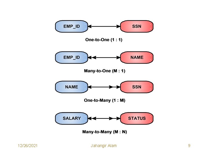
An Example • Consider the Entity “Employee”. • Attributes of this Entity may be – EMP_ID, SSN, Name, Salary, Address, Status etc. • Anyone among EMP_ID and SSN can be chosen as Primary Key (An attribute that is capable of uniquely identifying a given employee). • Some possible associations (relationships) among the attributes of Employee have been shown in the figure on the next page. 12/26/2021 Jahangir Alam 8

12/26/2021 Jahangir Alam 9

Relationships Among Entities • As associations (relationships) do exist between the attributes of a given entity, similarly two entities may also be related. • We distinguish between the association that exists among the attributes of an entity, called attribute association, and that which exists between entities, called a relationship. 12/26/2021 Jahangir Alam 10

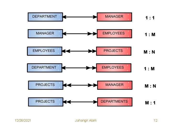
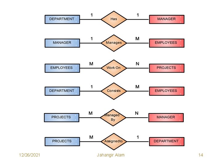
An Example: Employees in an organization work on several projects. Identify Entities and their relationships. • Possible Entities are: – – MANAGER EMPLOYEES DEPARTMENT PROJECTS • Relationships Among Entities: – – – Relationship between DEPARTMENT and MANAGER is 1 : 1. Relationship between MANAGER and EMPLOYEES is 1 : M. Relationship between EMPLOYEES and PROJECTS is M : N. Relationship between DEPARTMENT and EMPLOYEES is 1 : M. Relationship between PROJECTS and MANAGER M : N. Relationship between PROJECTS and DEPARTMENT is M : 1. 12/26/2021 Jahangir Alam 11

12/26/2021 Jahangir Alam 12

Conceptual Data Modeling Entity Relationship (E-R) Model • We analyze the organization and try to obtain an ER diagram (model). • We concentrate only on the relationships among entities and on the attributes of a single entity and not on the attributes associations. • An entity is shown as a rectangle. • A diamond represents the relationship among a number of entities which are connected to the diamond by lines. • The attributes shown as oval are connected to the entities or relationships by lines. • Diamonds, Ovals and rectangles are labeled. The type of relationship existing between the entities is represented by giving the type of the relationship on the lines joining the relationship to the entity. • The entities relationships shown in the above figure must be shown as below in the ER Diagram. 12/26/2021 Jahangir Alam 13

12/26/2021 Jahangir Alam 14

ER Diagram for Employees – Projects Problem Statement: • Several Employees in various Departments managed by different individual Managers work on several projects. Draw an ER diagram for modeling the data of organization. 12/26/2021 Jahangir Alam 15

12/26/2021 Jahangir Alam 16

Students – Teachers – Courses Problem Statement: • In a University department students are taught several courses by different teachers. Identify entities and draw an ER diagram to model the data of the department. 12/26/2021 Jahangir Alam 17

12/26/2021 Jahangir Alam 18

Problems 1. A machine shop produces many parts which it takes on contract. It has many machinists who can operate any of the machines. A part needs working on only one machine. A record is kept on the quality of material needed for producing each part. The production of each part is tracked by giving a job number, start time , end time and machinist identification. Obtain an ER diagram for this problem. 2. A magazine is published monthly and is sent by post to its subscribers. Two months before the expiry of subscription, a reminder is sent to the subscriber. If subscription is not within a month another reminder is sent. If renewal subscription received up to two weeks before the expiry of subscription the subscriber’s name is removed from the mailing list and the subscriber is informed. Obtain an ER diagram to model the situation. 12/26/2021 Jahangir Alam 19

3. A library receives 1300 journals of varying periodicities. The journals receipt have to be recorded and displayed. Action has to be taken when journals are not received in time or lost in mail. Unless request for replacement is sent quickly, it may not be possible to get replacement. Journals have to be ordered at different times during the year and subscriptions renewed in time. Late payment of subscriptions may lead to non availability of earlier issues or paying high amounts for those issues, . Draw an ER diagram for the problem. 4. An advertisement is issued giving essential qualifications for the course, the last date receipt of application form and a fee to be enclosed with the application. A clerk in the registrar’s office checks the received applications to see if marks sheet and fee are enclosed and sends valid … … … 12/26/2021 Jahangir Alam 20

applications to the concerned academic departments. The department checks the application in detail and decides the applicants to be admitted, those to be put in waiting list and those rejected. Appropriate letters are sent to the registrar’s office which intimates the applicants. Draw ER diagram for the problem. 5. Draw an ER diagram for a banking system. • … … 12/26/2021 … Jahangir Alam 21

Object Data Model • I am assuming that you are well aware of Object Oriented Design concepts, so presenting only a very brief overview of this model. • Like an ER model, the Object Oriented Model is based on collection of objects. An object contains values stored in instance variables within the object. An object also contains bodies of code (functions) that operate on the instance variables. These bodies of code are called member functions or methods. • Objects contain the same types of values and they are grouped into classes. A class may be viewed as a type definition for objects. This combination of data and methods comprising a type definition is similar to a programming language abstract data type. • The only way in which one object can access the data of another object is by invoking a method of that object. This is called sending a message to the object. 12/26/2021 Jahangir Alam 22

Representational (Traditional) Data Models Hierarchical Data Model • The Hierarchical Data Model (HDM) uses the tree concept to represent data and the relationships among data. • The nodes of the tree are the record types (segments) representing the entities and are connected by links. • Each hierarchical tree can have only one root record type and this record type doesn’t have a parent record type. • The root can have any number of child record types, each of which can itself be a root of another hierarchical tree. • Each child record type can have only one parent record type, thus a many to many relationship can’t be directly expressed between two record types. • Data in parent record applies to all its child records. A child record occurrence must have a parent record occurrence. 12/26/2021 Jahangir Alam 23

• Deleting a parent record occurrence requires deleting all its child record occurrences. • A hierarchical tree can have any number of record occurrences for each record type at each level of hierarchy. 12/26/2021 Jahangir Alam 24

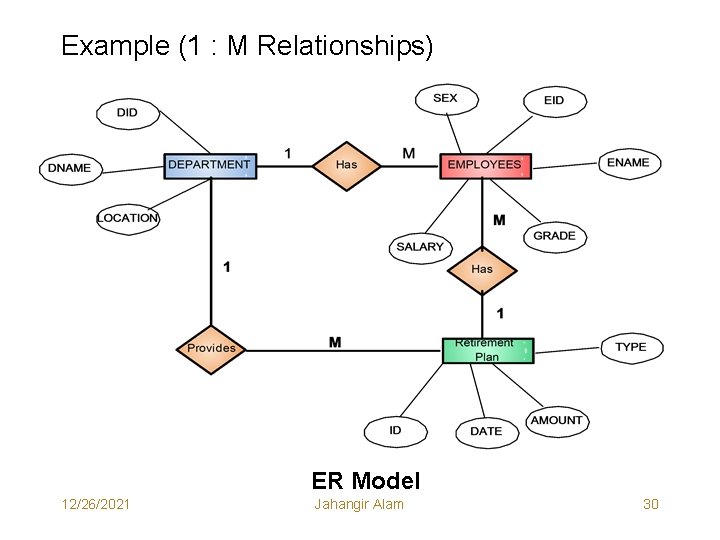
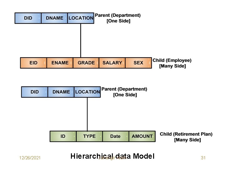
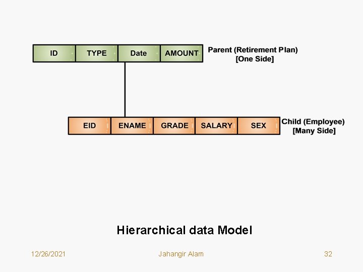
Transforming an ER Model to Hierarchical Data Structures (Hierarchical Model) 1. Transforming One to One Relationships: • We follow the following Rule: – For each entity E in the ER model, create a record type (segment) S in the hierarchical model. All attributes of E are represented as fields of S. Any of the segments may be chosen as parent and the other segment becomes the child. 2. Transforming One to Many Relationships: • We follow the following two Rules: – For each entity E in the ER model, create a record type (segment) S in the hierarchical model. All attributes of E are represented as fields of S. – For one to many relationship between two entities, create corresponding tree structure diagrams, making each entity as record type and making one to many relationship as a parent child relationship. The record type (segment) on the many side of the relationship becomes the child record type and the record type on the one side of the relationship becomes the parent. 12/26/2021 Jahangir Alam 25

3. Transforming Many to Many Relationships: • We follow the following two Rules: – For entities E 1 and E 2 that have a many to many relationship and from which segments (record types) S 1 and S 2 have been derived, construct two different trees: S 1 to S 2 and S 2 to S 1. In one tree S 1 would be parent and in the other tree it would be child. Similarly in one tree S 2 would be child and in the other tree it would be parent. – If a many to many relationship has common attribute data, create a new intersection segment I which contains that data. Each of the segment types created from the entities will function as a root of a distinct tree. Insert the new segment between the two entity types and establish the corresponding one to many relationships between parent child segments. If any of those parent child relationships are exactly one to one, the common attribute data might be combined into segments created from entities. 12/26/2021 Jahangir Alam 26

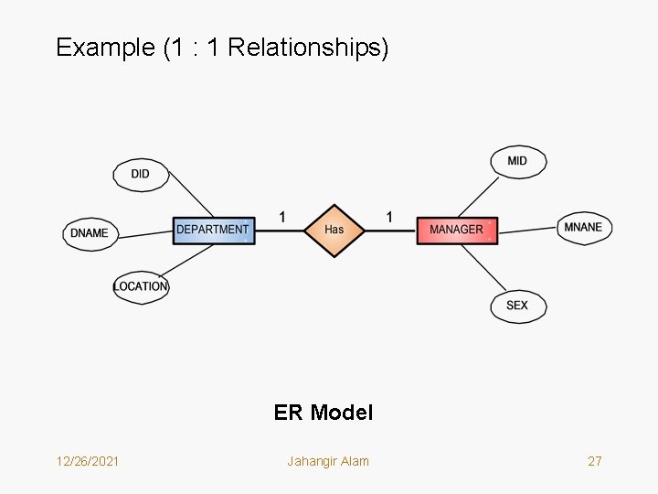
Example (1 : 1 Relationships) ER Model 12/26/2021 Jahangir Alam 27

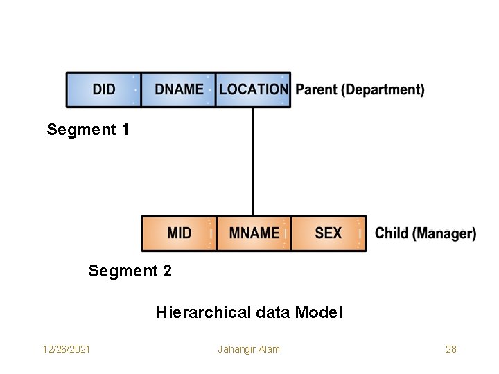
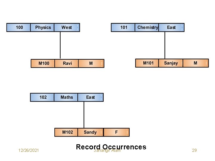
Segment 1 Segment 2 Hierarchical data Model 12/26/2021 Jahangir Alam 28

12/26/2021 Record Occurrences Jahangir Alam 29

Example (1 : M Relationships) ER Model 12/26/2021 Jahangir Alam 30

12/26/2021 Hierarchical Jahangirdata Alam Model 31

Hierarchical data Model 12/26/2021 Jahangir Alam 32

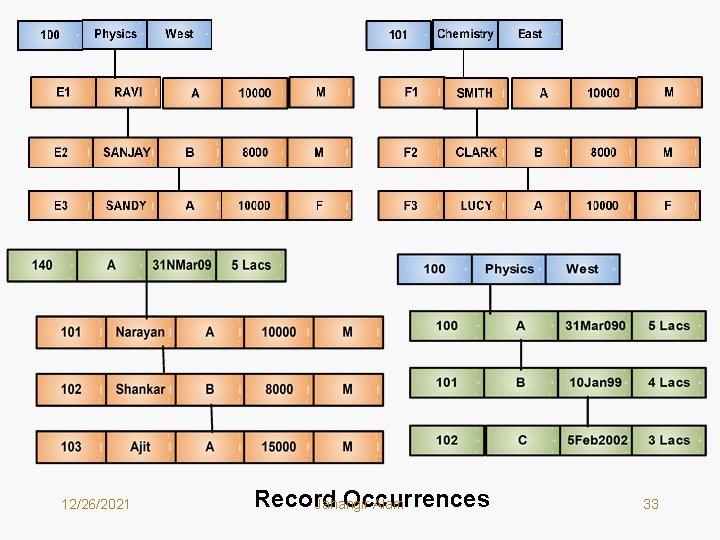
12/26/2021 Record Occurrences Jahangir Alam 33

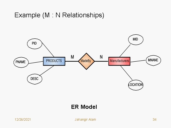
Example (M : N Relationships) ER Model 12/26/2021 Jahangir Alam 34

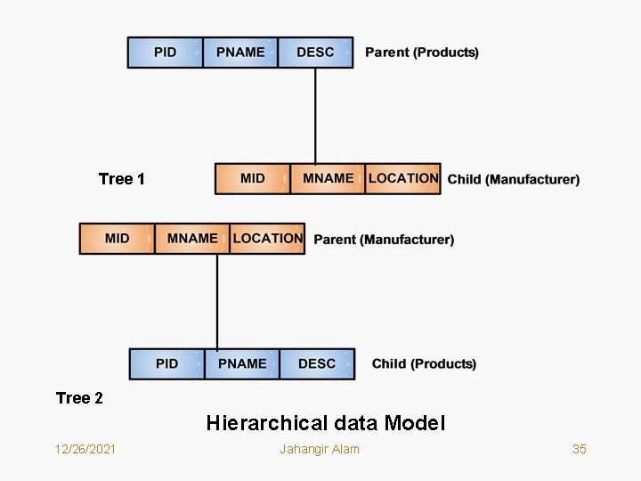
Tree 1 Tree 2 Hierarchical data Model 12/26/2021 Jahangir Alam 35

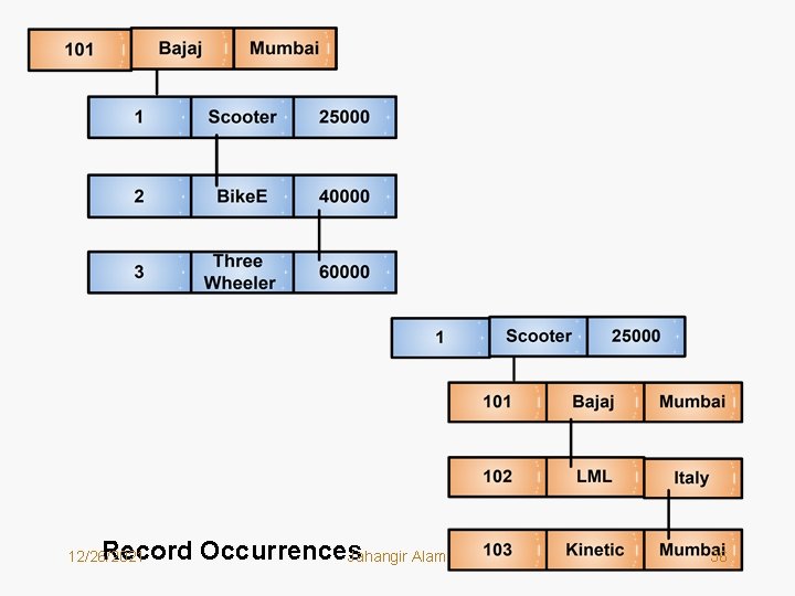
Record Occurrences Jahangir Alam 12/26/2021 36

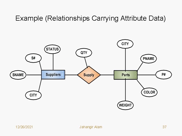
Example (Relationships Carrying Attribute Data) 12/26/2021 Jahangir Alam 37

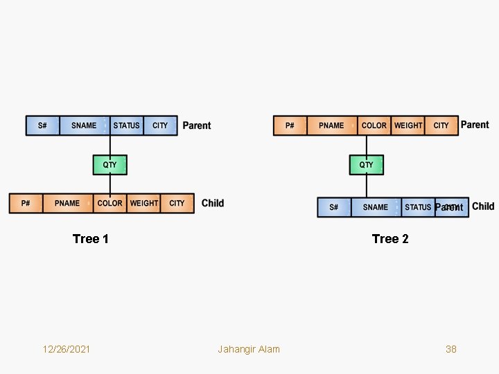
Tree 1 12/26/2021 Tree 2 Jahangir Alam 38

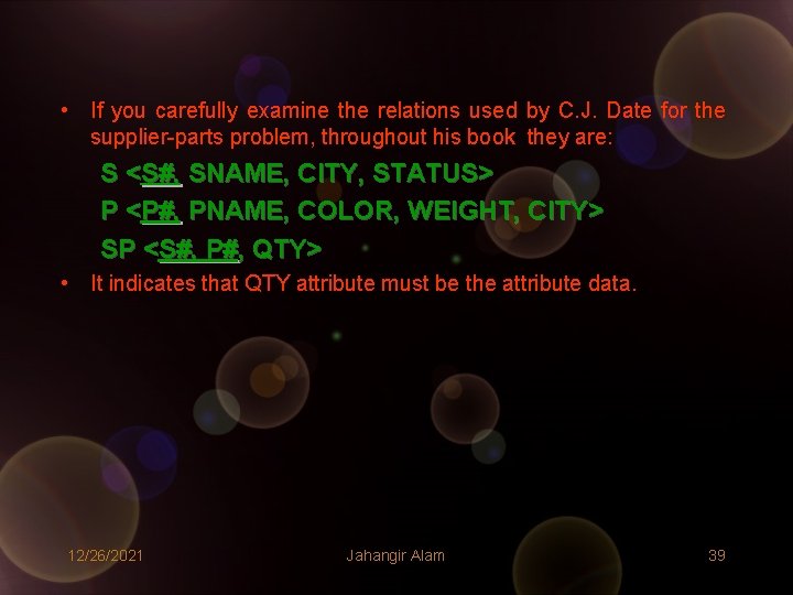
• If you carefully examine the relations used by C. J. Date for the supplier-parts problem, throughout his book they are: S <S#, SNAME, CITY, STATUS> P <P#, PNAME, COLOR, WEIGHT, CITY> SP <S#, P#, QTY> • It indicates that QTY attribute must be the attribute data. 12/26/2021 Jahangir Alam 39

Evaluation of Hierarchical Model • There are three features that define the hierarchical data structures – trees, segments and fields. • While any ER model can be transformed to a hierarchical data structure, the requirement that all database records can be trees may result in segments duplication. • Any situation whose natural mapping results in a segment being a child segment of two distinct parent segments requires that those parent segments occur in separate trees. • As an example consider the ER Model and its transformation to Hierarchical Data Structures, on the next page. • Such duplication has the following negative points: – Storage space is used inefficiently as the segment is repeated. – Possibility of inconsistent data is there, if the data are changed in one segment copy but not in the other. 12/26/2021 Jahangir Alam 40

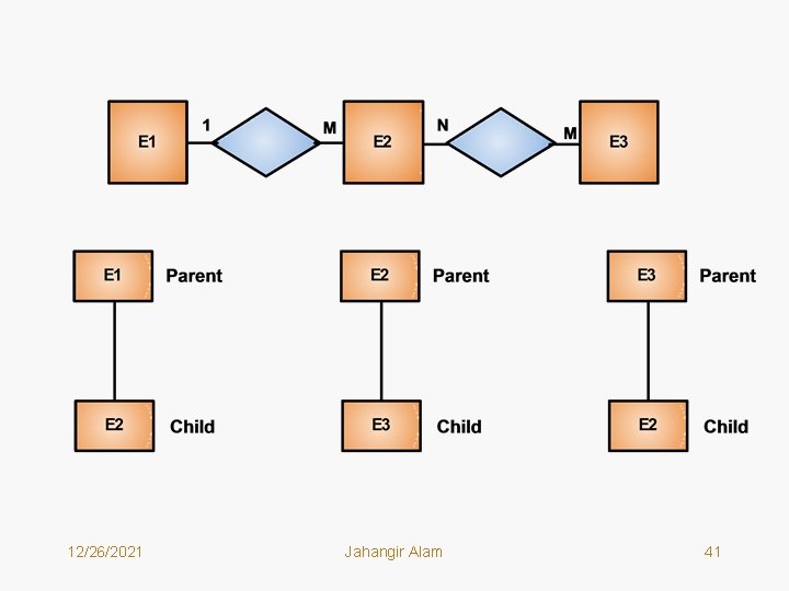
12/26/2021 Jahangir Alam 41

• This problem has been dealt with the help of virtual segments. A Virtual Segment contains no data but has a pointer to a data segment where data are stored. • When a segment is required to be replicated in two or more trees, the actual data are stored in just one of the trees. All other occurrences of that data segment will contain a pointer to the location where the actual data are stored. • This is shown in the figure on the next page. 12/26/2021 Jahangir Alam 42

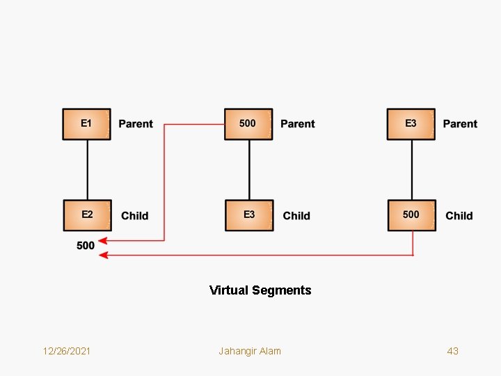
Virtual Segments 12/26/2021 Jahangir Alam 43

Examples of Commercial Database Management Systems Based on Hierarchical Approach • No DBMS supports hierarchical data organization in modern days. • Few legacy DBMSs based on this approach are: – IMS: IMS IBM’s Information Management System. It was once the leading DBMS based on Hierarchical approach. – TDMS: TDMS System Development Corporation’s Time Shared Data Management System. – Mark IV: IV Control Data Corporation’s Multi Access Retrieval System. – System 2000: 2000 SAS Institute’s Hierarchical DBMS. 12/26/2021 Jahangir Alam 44

Network Data Model • • • Networks are natural ways of representing relationships among objects. They are widely used in mathematics, chemistry, electrical engineering and in other fields. Networks are generally represented by a mathematical structure called a directed graph. Directed Graph has a simple structure and is constructed from points or nodes connected by arrows or edges. In the concepts of data models nodes can be thought of as data record types (or segments) and networks can be thought of as representing one to one or one to many relationships. Clearly, Network Data Model represents structures of records types (segments) connected in one to one or one to many relationships. The graph structure enables simple representation of relationships between objects and moreover once a relationship has been established between two objects, retrieval and manipulation of the related data can be efficiently done. Network Data Model is also called CODASYL DBTG Model or simply DBTG model. 12/26/2021 Jahangir Alam 45

Terminology of Network Data Model • There are two fundamental data structures in Network data Model: – Record Types (same as Segments in Hierarchical Data Model) – Sets • Record Types are defined in a usual way as collections of logically related data items (fields). Record types are same as segments in hierarchical model. • DBTG Set or simply Set in the DBTG model expresses a one to one or one to many relationship between two record types (segments) or entities. The record type on the one side of the one to many relationship of a DBTG set is called the Owner record type and the record type on the many side of the one to many relationship of a DBTG set is called Member record type. In a one to one relationship any record type can be chosen as Owner and the other becomes the member. 12/26/2021 Jahangir Alam 46

Transforming an ER Model to Network Data Structures (Network Model) • • • Conceptual (ER) modeling to network data modeling is expressed by means of Batchman Diagrams. Following conventions are there for constructing the Batchman Diagrams: – The sets are denoted by the arrows between the record types with the arrow pointing to the member record type. – Each set is consists of an owner record type, a member record and a name for the set. The set name is the label given to the arrow. Simple & Complex Networks: A conceptual data structure (ER Model) in which all relationships are one to one or one to many is called a Simple Network and a conceptual data structure in which one or more relationships are many to many is called Complex Network. Note that the DBTG network model allows only simple networks in which all relationships are one to many or one to one. A complex network can’t be directly implemented in DBTG model. 12/26/2021 Jahangir Alam 47

Rules for Transformation 1. Transforming One to One Relationships: • We follow the following Rule: – For each entity E in the ER model, create a record type R in the network model. All attributes of E are represented as fields of R. Any of the record types may be chosen as owner and the other record type becomes the member. 2. Transforming One to Many Relationships: • We follow the following Rules: – For each entity E in the ER model, create a record type R in the network model. All attributes of E are represented as fields of R. – For one to many relationship the record type on one side of the relationship becomes the owner and the record type on the many side of the relationship becomes the member. 12/26/2021 Jahangir Alam 48

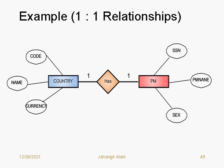
Example (1 : 1 Relationships) 12/26/2021 Jahangir Alam 49

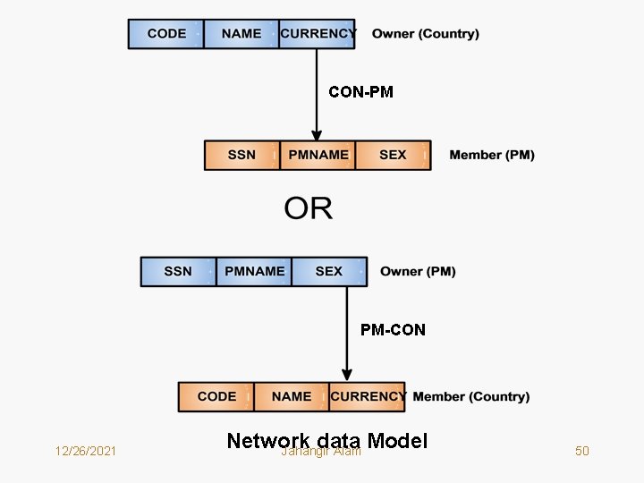
CON-PM PM-CON 12/26/2021 Network data Model Jahangir Alam 50

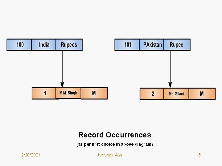
Record Occurrences (as per first choice in above diagram) 12/26/2021 Jahangir Alam 51

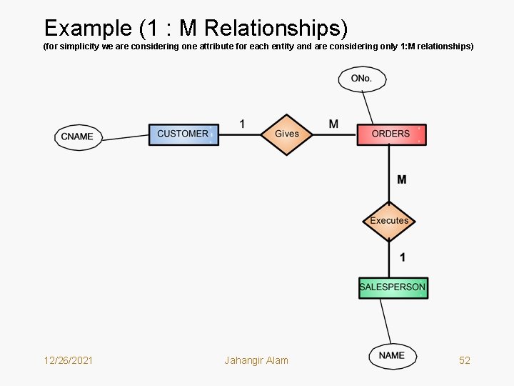
Example (1 : M Relationships) (for simplicity we are considering one attribute for each entity and are considering only 1: M relationships) 12/26/2021 Jahangir Alam 52

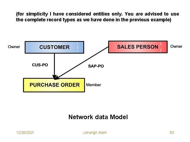
(for simplicity I have considered entities only. You are advised to use the complete record types as we have done in the previous example) Network data Model 12/26/2021 Jahangir Alam 53

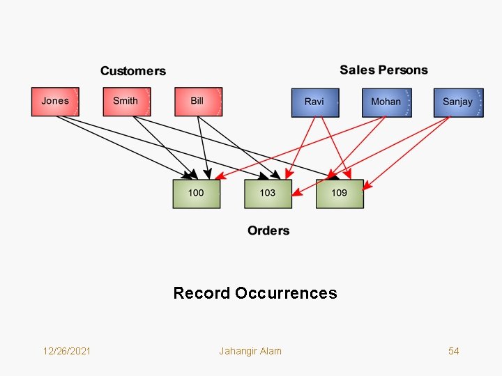
Record Occurrences 12/26/2021 Jahangir Alam 54

3. Transforming Manyto Many Relationships: • When two entities are connected in many to many relationship we create an intersection or link record type consisting of at least the key attributes from both the entities. Other attributes may be added at the discretion of the designer. • What is a link record? – A dummy record type that is created in order to convert a complex network into an equivalent simple network is called a link record or link record type. – With the creation of link record type, all many to many relationships are converted into equivalent one to many relationships. Which are required by the DBTG Network Model. • So, to derive the Network Data Structure, we follow the following rule: – For each many to many relationship between entities E 1 and E 2, create a link record type L, and make it the member record type in the two set types, of which the set types owners are the record types corresponding to E 1 and E 2. 12/26/2021 Jahangir Alam 55

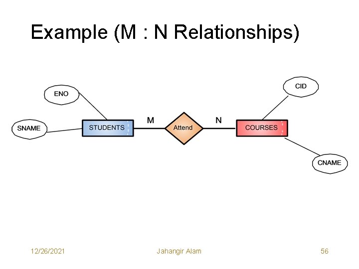
Example (M : N Relationships) 12/26/2021 Jahangir Alam 56

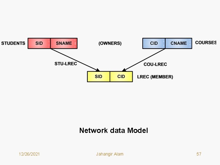
Network data Model 12/26/2021 Jahangir Alam 57

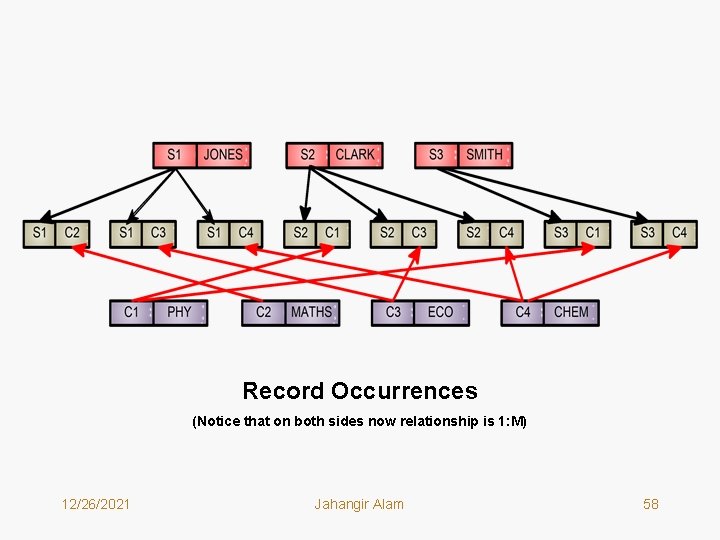
Record Occurrences (Notice that on both sides now relationship is 1: M) 12/26/2021 Jahangir Alam 58

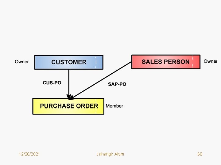
Hierarchical Vs. Network Data Model • Consider the Network Data Structure shown on the next page for the Customer-Sales Person-Purchase problem. • This example indicates the clear difference between hierarchical and network models. • In this figure, the PURCHASE ORDER record type is a member (Child) of two sets (Parents) – CUS-PO and SAP-PO. • In the hierarchical data model no record type can be a member (child) of two different sets (parents). 12/26/2021 Jahangir Alam 59

12/26/2021 Jahangir Alam 60

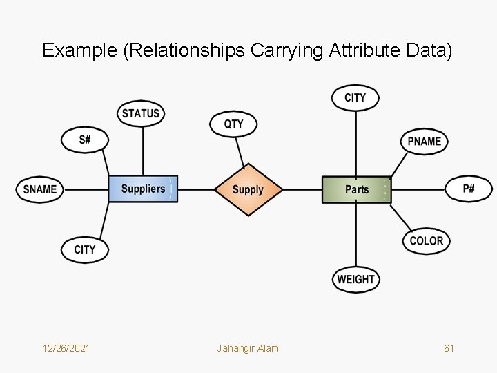
Example (Relationships Carrying Attribute Data) 12/26/2021 Jahangir Alam 61

SOLUTION… Key to solution is that the attribute data is included with the LINK RECORD TYPE. 12/26/2021 Jahangir Alam 62

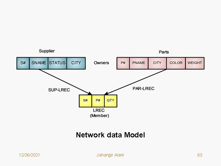
Network data Model 12/26/2021 Jahangir Alam 63

Examples of Commercial Database Management Systems Based on Hierarchical Approach • No DBMS supports network data organization in modern days. • Few legacy DBMSs based on this approach are: – IDMS/ R: The most widely used commercial implementation of DBTG network data model. It stands for Integrated Database Management System/ Relational – DMS 1100: 1100 from UNIVAC. – TOTAL: TOTAL from Cincom’s. – DBDMP: DBDMP (Database Operations & Manipulation Process) from IBM. 12/26/2021 Jahangir Alam 64

Relational Data Model • In 1970 the way many people viewed databases was permanently changed when E. F. Codd introduced the relational model. • In this model relation is the only construct required to represent the associations among the attributes of an entity as well as the relationships among different entities. • One of the major reasons for introducing this model was to increase the productivity of application programmers by eliminating the need to change application programs when a change is made to the database. Users need not to know the exact physical structure to use the database. They are however required to know how the data has been partitioned into various relations. • In relational data model, relation is the only data structure used to represent entities and relationships among them. 12/26/2021 Jahangir Alam 65

• In addition Codd proposed two data languages which promised more power in accessing and processing the data. These Languages are: – Relational Algebra – Relational Calculus • Today, these languages provide the basis for the commercial database languages used in many of the most popular commercial DBMSs. 12/26/2021 Jahangir Alam 66

Terminology of Relational Model Relation: Given a collection of sets D 1, D 2 , D 3 …. …. …. Dn, R is a relation on those n sets if it is a set of ordered n-tuples < d 1, d 2 , d 3 …. …. …. dn> such that d 1є D 1, d 2є D 2, d 3є D 3, ……. , dnє Dn. Sets D 1, D 2 , D 3 …. …. …. Dn are called the domains of R and the value n is called the degree of R. OR We define R to be relation on sets D 1, D 2 , D 3 …. …. …. Dn, if it is a subset of the Cartesian Product D 1 X D 2 X D 3 …. …. …. X Dn, Cartesian product of these n sets, written as “D 1 X D 2 X D 3 …. …. …. X Dn” is the set of all possible ordered n tuples < d 1, d 2 , d 3 …. …. …. dn> such d 1є D 1, d 2є D 2, d 3є D 3, ……. , dnє Dn. 12/26/2021 Jahangir Alam 67

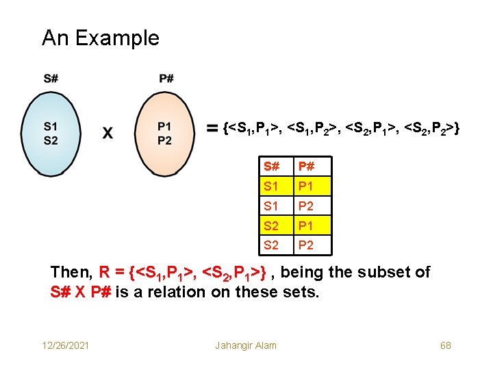
An Example {<S 1, P 1>, <S 1, P 2>, <S 2, P 1>, <S 2, P 2>} S# P# S 1 P 1 S 1 P 2 S 2 P 1 S 2 P 2 Then, R = {<S 1, P 1>, <S 2, P 1>} , being the subset of S# X P# is a relation on these sets. 12/26/2021 Jahangir Alam 68

• Clearly, a relation represents a unique two dimensional table consisting of rows and columns of data. • Thus relational model organizes and represents the data in the form of tables (the two dimensional data structure). Cardinality of a Relation: • The number of rows (tuples) in a relation is called the cardinality of the relation. • We have already defined the degree of a relation. Relations of degree one are called unary relations, that of degree two are called binary relations, that of degree three are called ternary relations and so on. • A relation of degree n is called n-ary relation. 12/26/2021 Jahangir Alam 69

Domains and Attributes: • Each column in a relation is an attribute of the relation. For example in our relation S# and P# are attributes. • The set of all possible values that an attribute may have is called the domain of attribute. • Every attribute in a relation is defined on a domain. Domains may be distinct for each attribute or two or more attributes may be defined on the same domain. • Note that at any given instant of time there will be values in the domain that do not currently appear as values in the corresponding attribute. Tuples: • The rows of a relation are called tuples. It is assumed that there is no predefined order of the rows or tuples of a relation and that no two tuples can have identical set of values. 12/26/2021 Jahangir Alam 70

Recursive Relationship: • To understand the concept of recursive relationship, consider the ER diagram on the next page. • A relationship which relates an object set or an entity set to itself is called the recursive relationship. • For example in the following diagram the relationship, “supervises “ is a recursive relationship. • We can derive the following relations from the ER diagram in question: WORKER<WORKER_ID, NAME, HOURLY_RATE, SKILL_TYPE, SUPV_ID> ASSIGNMENT<WORKER_ID, BUILD_ID, START_DATE, NUM_DAYS> BUILDING<BUILD_ID, BUILD_ADDRESS, TYPE, QUALITY_LEVEL, STATUS> SKILL<SKILL_TYPE, BONOUS_RATE, HOURS_PER_WEEK> 12/26/2021 Jahangir Alam 71

12/26/2021 Jahangir Alam 72

NULL Values: • Suppose an attribute is not applicable in a specific case. For example some employees in the WORKER relation don’t have supervisors (or they themselves are supervisors). • In that case no value exists corresponding to SUPV_ID attribute for such employees. • In addition when we are entering data for a row in a relation, we might not know the values of one or more of the attributes for that row. • In either case we enter nothing, and the row is recorded in the database with null values for those attributes. • A null value is neither a blank nor a zero. • It is simply unknown and may be supplied at a later time. 12/26/2021 Jahangir Alam 73

Terminology of Relational Keys • A key is a single attribute or combination of two or more attributes of a relation that is used to uniquely identify a tuple in the relation. • For example in the Worker relation, the WORKER_ID attribute is a key. When we refer to the term key, we normally mean to primary key. • Here we concentrate on the terminology used for relational keys. Superkey: • If we additional attribute to a key (primary key) and the resulting combination of attributes still uniquely identifies a tuple in the relation, it is called a superkey of the relation. • For example the combination (WORKER_ID, Name) uniquely identifies each worker in the WORKER relation, so it is a superkey of the relation. • Clearly, a key of a relation is a minimal set of such attributes. 12/26/2021 Jahangir Alam 74

• That is, a key is a minimal superkey. By minimal we mean that no subset of the set of key attributes will uniquely identify tuples in the relation. • As an example consider the relation SP<S#, P#, QTY> Key to the relation is (S#, P#). If we add an additional attribute i. e. QTY with this attributes combination, we get the superkey of the relation as (S#, P#, QTY). Clearly key is the minimal set of attributes that uniquely identify each row in the relation. No subset of the key attributes (i. e. S# or P# individually) can be used as key. Composite Key: • A key consisting of more than one attribute is called a composite key. • For example in the ASSIGNMENT relation the attributes combination (WORKER_ID, BUILD_ID) uniquely identifies each tuple in the relation, so key to the relation is composite. • In the same manner the attributes combination (S#, P#) is the composite key to SP relation. 12/26/2021 Jahangir Alam 75

Candidate Keys: • In any given relation there may be more than one set of attributes that could be chosen as a key. These are called candidate keys. • It may appear for example that NAME is a candidate key in the WORKER relation. This would be so if we could assume that NAME will always be unique. Primary Key: • When one of the candidate keys is selected as the relational key, it is called the Primary Key. • The remaining candidate keys would be considered as alternate keys. • When we use the term key we mean to primary key. Secondary Key: • A secondary key is an attribute or combination of attributes that may not be a candidate key but that classifies the relation based on a particular characteristics (or criteria). 12/26/2021 Jahangir Alam 76

• • Actually, a secondary key is one that identifies a set of records having the same values for the secondary key attribute. For example in the relation WORKER, the SKILL_TYPE attribute is a secondary key when the following query is executed: select NAME, WORKER_ID from WORKER where SKILL_TYP E= ‘ Engg. ”; Foreign Key: • A foreign key is a set of attributes (or single attribute) in a relation • that is a primary key in another relation (or in the same relation). For example, SKILL_TYPE attribute in the WORKER relation and BUILD_ID attribute in the ASSIGNMENT relation are foreign keys as they are primary keys in the relations SKILL and BULIDING respectively. Importance of Foreign Keys: • Foreign keys are the essential links between relations. They are used • to tie data in one relation to the data in another relation. Thus SKILL_TYPE links the WORKER relation to the SKILL relation and BUILD_ID in the ASSIGNMENT relation show the link between WORKER and BUILDING relations. 12/26/2021 Jahangir Alam 77

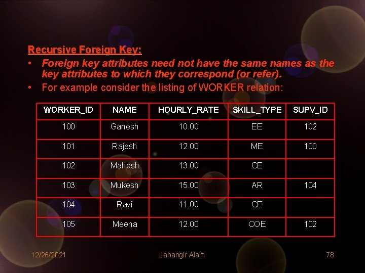
Recursive Foreign Key: • Foreign key attributes need not have the same names as the key attributes to which they correspond (or refer). • For example consider the listing of WORKER relation: WORKER_ID NAME HOURLY_RATE SKILL_TYPE SUPV_ID 100 Ganesh 10. 00 EE 102 101 Rajesh 12. 00 ME 100 102 Mahesh 13. 00 CE 103 Mukesh 15. 00 AR 104 Ravi 11. 00 CE 105 Meena 12. 00 COE 12/26/2021 Jahangir Alam 104 102 78

• Both WORKER_ID and SUPV_ID in the WORKER relation have different names but both take their values from the same domain (i. e. the domain of workers identification numbers). • The SUPV_ID is a foreign key in the worker relation that references the key of its own relation. Such foreign keys are called Recursive Foreign Keys. • Thus a recursive foreign key is nothing but a foreign key that references the key of its own relation. 12/26/2021 Jahangir Alam 79

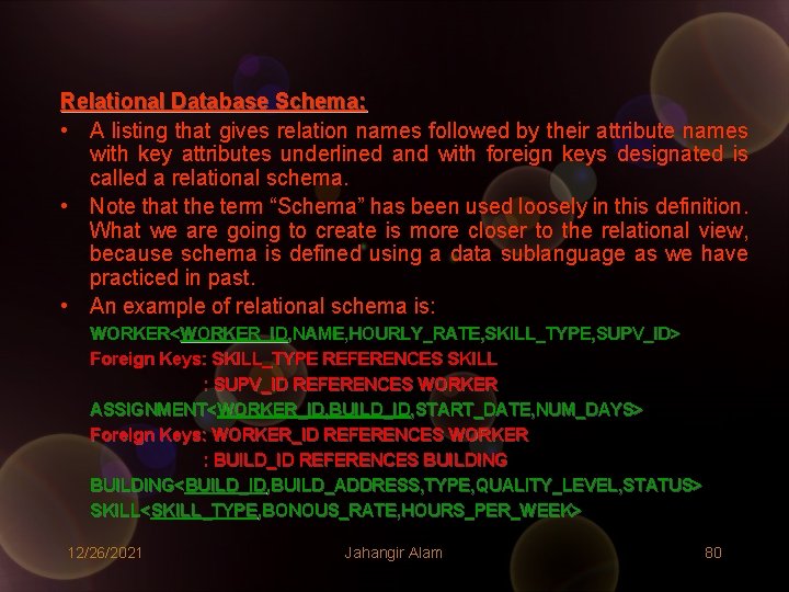
Relational Database Schema: • A listing that gives relation names followed by their attribute names with key attributes underlined and with foreign keys designated is called a relational schema. • Note that the term “Schema” has been used loosely in this definition. What we are going to create is more closer to the relational view, because schema is defined using a data sublanguage as we have practiced in past. • An example of relational schema is: WORKER<WORKER_ID, NAME, HOURLY_RATE, SKILL_TYPE, SUPV_ID> Foreign Keys: SKILL_TYPE REFERENCES SKILL : SUPV_ID REFERENCES WORKER ASSIGNMENT<WORKER_ID, BUILD_ID, START_DATE, NUM_DAYS> Foreign Keys: WORKER_ID REFERENCES WORKER : BUILD_ID REFERENCES BUILDING<BUILD_ID, BUILD_ADDRESS, TYPE, QUALITY_LEVEL, STATUS> SKILL<SKILL_TYPE, BONOUS_RATE, HOURS_PER_WEEK> 12/26/2021 Jahangir Alam 80

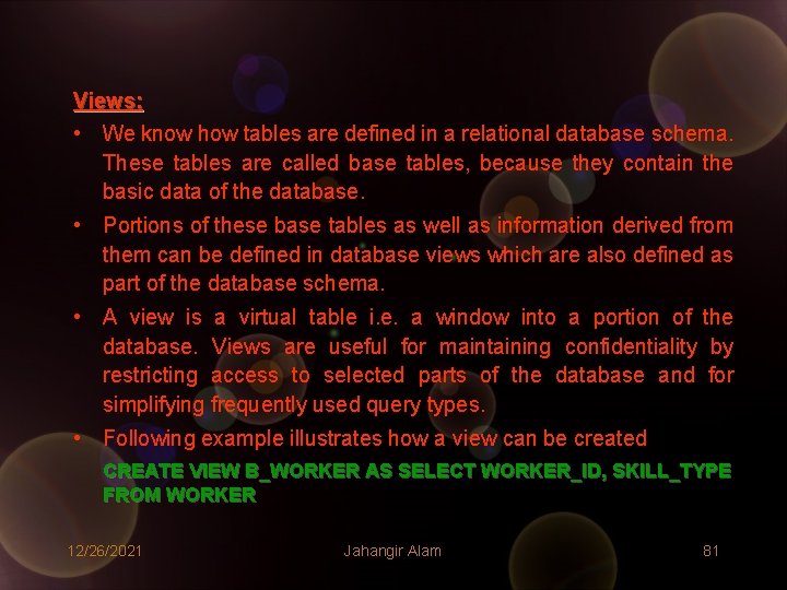
Views: • We know how tables are defined in a relational database schema. These tables are called base tables, because they contain the basic data of the database. • Portions of these base tables as well as information derived from them can be defined in database views which are also defined as part of the database schema. • A view is a virtual table i. e. a window into a portion of the database. Views are useful for maintaining confidentiality by restricting access to selected parts of the database and for simplifying frequently used query types. • Following example illustrates how a view can be created CREATE VIEW B_WORKER AS SELECT WORKER_ID, SKILL_TYPE FROM WORKER 12/26/2021 Jahangir Alam 81

Constraints: • A constraint is a rule that restricts the values that may be present in • the database. Codd’s relational model include several constraints, which are used to verify the validity of data in a database as well as to add meaningful structure to the data. These constraints are called Codd’s Rule for RDBMs. Codd’s rules are also used to verify “When a DBMS is Relational? ” • • Codd’s Rule for RDBMS: 1. Information Rule: All information in a database including table name, column names etc. are represented explicitly by values in tables. 2. Guaranteed Access Rule: Every piece of data in a relational database can be accessed by using a combination of a table name, a primary key value that identifies the row and a column name that identifies the cell. 12/26/2021 Jahangir Alam 82

3. Systematic Treatment of Null Values: The RDBMS handles records that have unknown or inapplicable values in a predefined fashion. Also, RDBMS distinguishes between zeros, blanks and nulls in records and handles such values in a consistent manner that produces correct answers, comparisons and calculations. 4. Active On-Line Catalogue Based on Relational Model: The description of a database and its contents are database tables and therefore can be queried online via data language. 5. Comprehensive Data Sublanguage: The RDBMS may support several languages but at least one of them should allow the user to do all of the following: – – – Define Tables/ Views Query and Update Data Set Integrity Constraints Set Authorization Define Transactions 12/26/2021 Jahangir Alam 83

6. View Updating Rule: Any view that is theoretically updatable can be updated using RDBMS. A view is theoretically updatable if changes can be made to the tables that effect the desired changes in the view. By this facility data consistency is assured since changes in the underlying tables are transmitted in the view they support. 7. Higher Level Insert, Update and Delete: The RDBMS supports insertion, deletion and updating of data at a table level. 8. Physical Data Independence: The execution of ad-hoc requests and application programs is not effected by changes in the physical data access and storage media. 9. Logical Data Independence: Logical changes in tables and views such as adding/ deleting columns or changing field lengths do not require modifications in application programs or in the format of data reports. 12/26/2021 Jahangir Alam 84

10. Distribution Independence: Application programs and ad-hoc requests are not effected by changes in the distribution of physical data. 11. Integrity Independence: Like table/ view definitions integrity constraints are stored in the on-line catalogue and therefore can be changed without making changes in the application programs or in the format of the ad-hoc requests. Additionally integrity constraints can’t be by passed. Integrity constraints specific to a particular relational database must be definable in the relational data sublanguage and storable in the catalogue (not in the application program). At least the following two integrity constraints must be supported: – Integrity Rule 1 (Entity Integrity): If attribute A of relation R is a prime attribute (Primary Key) then A can’t accept NULL values. 12/26/2021 Jahangir Alam 85

If any attribute value of a primary key (prime attribute) were permitted to have null values then because the attribute values in key must be non – redundant, the key can’t be used for unique identification of tuples. - Integrity Rule 2 (Referential Integrity): Given two relations R and S, suppose R, refers to S via a set of attributes that forms the primary key of S. Clearly, this set of attributes forms a foreign key in R. Then, the values of the foreign key in a tuple in R must either be equal to the primary key of a tuple of S or entirely be NULL. As we know that in constructing relations foreign keys are used to tie rows in one relation to the rows in another relation. For example SKILL_TYPE is used in WORKER relation to tell us the principal skill of each employee so that the bonus pay rates may be calculated. Therefore it is extremely important that the value of SKILL_TYPE in any employee’s row corresponds to actual SKILL_TYPE value in the SKILL relation, otherwise the employee skill type would point nowhere. A database in which all non null foreign key values reference actual key values in other relations observes referential integrity. 12/26/2021 Jahangir Alam 86

12. Non Subversion Rule: If the RDBMS has a language that accesses the information of a record at a time, this language can’t be used to bypass the integrity constraints. In order to follow this rule the RDBMS must have an active catalogue that contains the constraints. 12/26/2021 Jahangir Alam 87

Transforming E-R Diagrams into Relational Data Structures (Model) • Please refer to the class notes. 12/26/2021 Jahangir Alam 88

Normalization • This topic is concerned with the design and implementation issues, that would be considered in a RDBMS (i. e. when we shall design a database using relation DBMS). • This is actually in continuation of our earlier discussion on RDBMS to further refine our design (View) to produce the relations in a form that is least prone to the problems like inconsistency and redundancy. • In general the goal of a relational database design is to generate a set of relational schema that allows us to store information without unnecessary redundancy, yet allows us to retrieve information easily. 12/26/2021 Jahangir Alam 89

What is Normalization? • The entities and their attributes can be organized into a set of tables in many different ways. • One method of organization is to design schemas that are in appropriate normal form. The theory behind such arrangement of attributes in tables is known as the Normalization. • The normalization of data helps to ensure that a particular organization conforms to such standards as: – Minimization of duplication of data (redundancy). – Providing flexibility to support different functional requirements. – Easy and consistent modification of data. – Enabling the organization to be translated to the actual database design. • A number of normal forms have been defined for classifying relations. Each normal form has associated with it a number of constraints. • A relational schema is said to be in a particular normal form if it satisfies all the constraints required for that normal form. 12/26/2021 Jahangir Alam 90

12/26/2021 Jahangir Alam 91

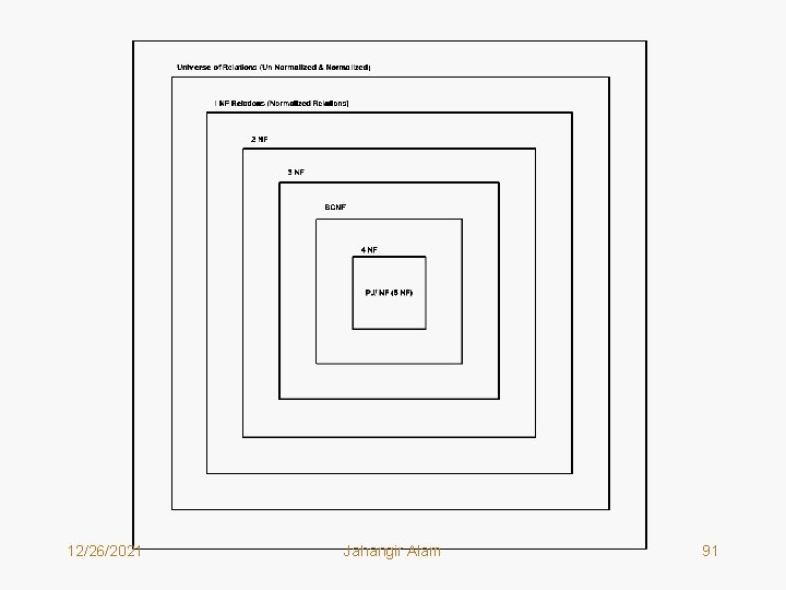
• In general if a given relation is in (n+1)th Normal form, it is obvious that the relation is in the nth Normal form. 12/26/2021 Jahangir Alam 92

Why do we Normalize Relations? Relations are normalized so that when relations in a database are to be altered during the lifetime of the database, we don’t loose vital information or introduce inconsistencies. The types of alterations normally needed for relations are: Insertion: • Insertion of data items into database should be possible without being forced to leave blank fields for some attributes. If our design has such undesirable property it is called Insertion Anomaly. Deletion: • Deletion of a tuple from a relation should be possible without loosing vital information. If our design has such undesirable property it is called Deletion Anomaly. Updation: • Updation or changing the value of an attribute should be possible without introducing inconsistencies in the database. If our design has such undesirable property it is called Updation Anomaly. Clearly Normalization is used to avoid anomalies from the design. 12/26/2021 Jahangir Alam 93

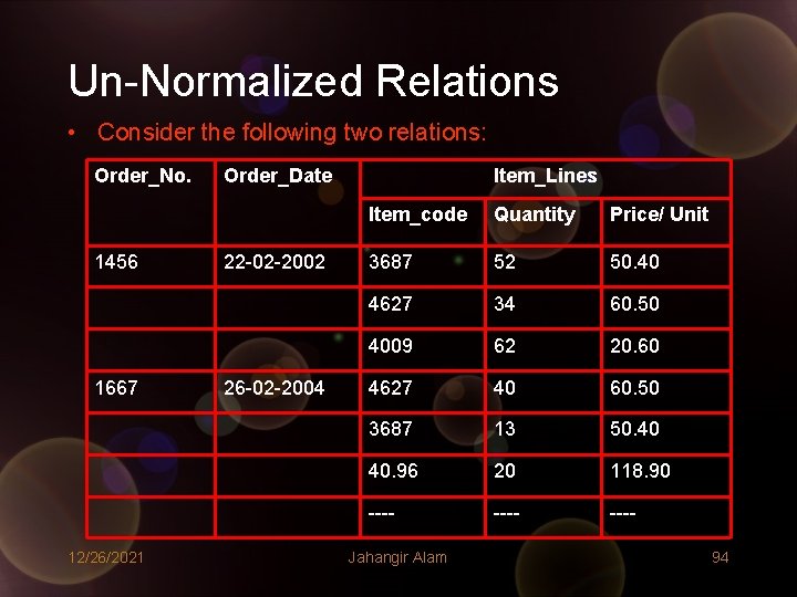
Un-Normalized Relations • Consider the following two relations: Order_No. 1456 1667 12/26/2021 Order_Date 22 -02 -2002 26 -02 -2004 Item_Lines Item_code Quantity Price/ Unit 3687 52 50. 40 4627 34 60. 50 4009 62 20. 60 4627 40 60. 50 3687 13 50. 40 40. 96 20 118. 90 ---- Jahangir Alam 94

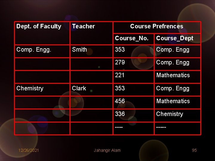
Dept. of Faculty Comp. Engg. Chemistry 12/26/2021 Teacher Smith Clark Course Prefrences Course_No. Course_Dept 353 Comp. Engg 279 Comp. Engg 221 Mathematics 353 Comp. Engg 456 Mathematics 336 Chemistry ----- Jahangir Alam 95

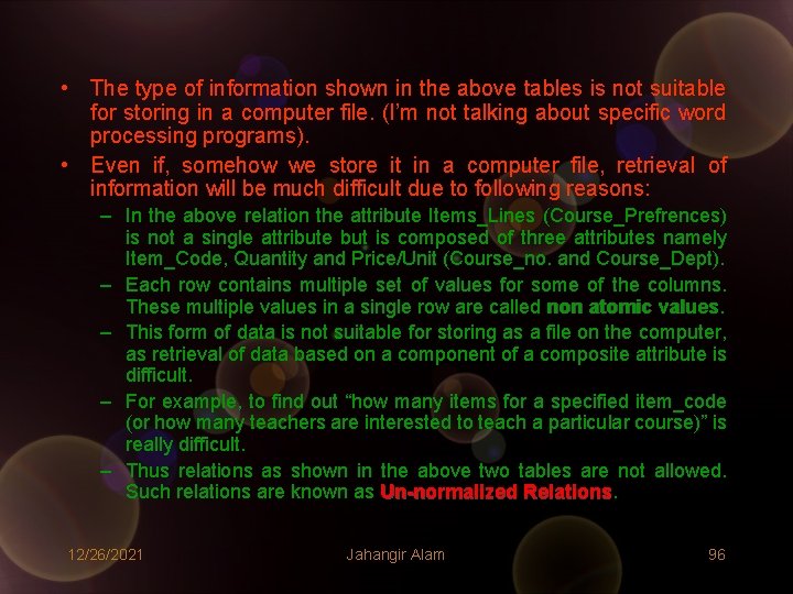
• The type of information shown in the above tables is not suitable for storing in a computer file. (I’m not talking about specific word processing programs). • Even if, somehow we store it in a computer file, retrieval of information will be much difficult due to following reasons: – In the above relation the attribute Items_Lines (Course_Prefrences) is not a single attribute but is composed of three attributes namely Item_Code, Quantity and Price/Unit (Course_no. and Course_Dept). – Each row contains multiple set of values for some of the columns. These multiple values in a single row are called non atomic values – This form of data is not suitable for storing as a file on the computer, as retrieval of data based on a component of a composite attribute is difficult. – For example, to find out “how many items for a specified item_code (or how many teachers are interested to teach a particular course)” is really difficult. – Thus relations as shown in the above two tables are not allowed. Such relations are known as Un-normalized Relations 12/26/2021 Jahangir Alam 96

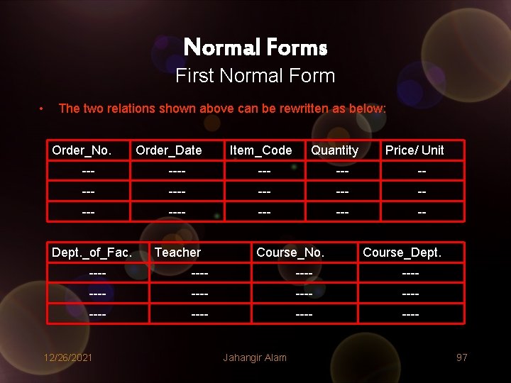
Normal Forms First Normal Form • The two relations shown above can be rewritten as below: Order_No. Order_Date Item_Code Quantity Price/ Unit --- ---- --- ---- --- -- Dept. _of_Fac. Teacher Course_No. Course_Dept. ---- ---- ---- 12/26/2021 Jahangir Alam 97

• The relations shown in the above two tables are called normalized relations and they are in First Normal Form. • Note that they don’t have any composite attribute i. e. values in each row are atomic. • So – “A Relation is in First Normal Form (1 NF) if and only if (iff) all underlying domains contain atomic values only. ” • A database schema is in 1 NF if and only if, every relation included in the database schema is in 1 NF. • Further discussion on Normalization requires the knowledge of Functional Dependencies as the higher normal forms are constrained by Functional Dependencies. 12/26/2021 Jahangir Alam 98

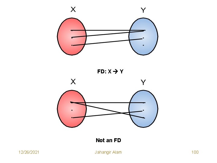
Functional Dependencies • Given a relation R, attribute Y of R is functionally dependent on attribute X of R if and only if, each X-value in R has associated with it precisely one Y-value in R. OR • Given a relation R, attribute Y of R is functionally dependent on attribute X of R, iff, whenever two tuples of R agree on their X-value, they also agree on their Y-value. • The notion for FD is: FD: R. X R. Y • The attribute on the left hand side of an FD is called determinant, because it determines the value of the attribute on the right hand side of the FD. • The above notion for FD is read as : “Attribute Y of R is functionally dependent on attribute X of R” or “Attribute X of R functionally determines attribute Y of R”. 12/26/2021 Jahangir Alam 99

FD: X Y Not an FD 12/26/2021 Jahangir Alam 100

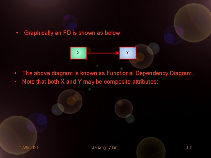
• Graphically an FD is shown as below: • The above diagram is known as Functional Dependency Diagram. • Note that both X and Y may be composite attributes: 12/26/2021 Jahangir Alam 101

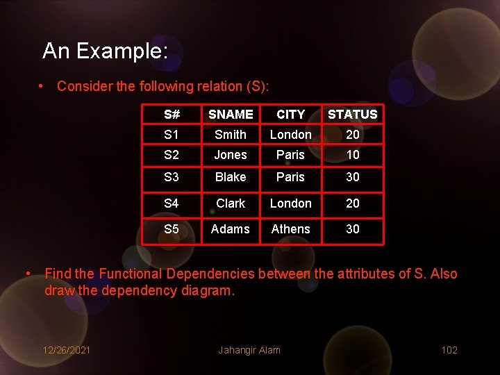
An Example: • Consider the following relation (S): S# SNAME CITY STATUS S 1 Smith London 20 S 2 Jones Paris 10 S 3 Blake Paris 30 S 4 Clark London 20 S 5 Adams Athens 30 • Find the Functional Dependencies between the attributes of S. Also draw the dependency diagram. 12/26/2021 Jahangir Alam 102

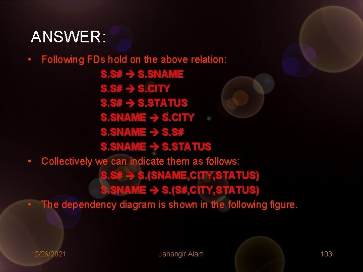
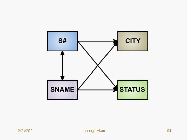
ANSWER: • Following FDs hold on the above relation: S. S# S. SNAME S. S# S. CITY S. S# S. STATUS S. SNAME S. CITY S. SNAME S. S# S. SNAME S. STATUS • Collectively we can indicate them as follows: S. S# S. (SNAME, CITY, STATUS) S. SNAME S. (S#, CITY, STATUS) • The dependency diagram is shown in the following figure. 12/26/2021 Jahangir Alam 103

12/26/2021 Jahangir Alam 104

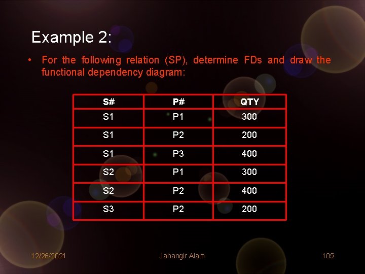
Example 2: • For the following relation (SP), determine FDs and draw the functional dependency diagram: 12/26/2021 S# P# QTY S 1 P 1 300 S 1 P 2 200 S 1 P 3 400 S 2 P 1 300 S 2 P 2 400 S 3 P 2 200 Jahangir Alam 105

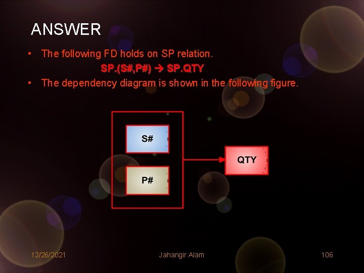
ANSWER • The following FD holds on SP relation. SP. (S#, P#) SP. QTY • The dependency diagram is shown in the following figure. 12/26/2021 Jahangir Alam 106

Full Functional Dependency • Given a relation R and an FD: R. X R. Y. Attribute Y of R is fully functionally dependent on attribute X of R, if there is no Z, where Z is a proper subset of X, such that Z determines Y. • So, full functional dependency is meaningful when X is a composite attribute, otherwise functional dependency and full functional are used interchangeably. 12/26/2021 Jahangir Alam 107

An Example: • Consider the relation S. Determine whether S. CITY is fully functionally dependent upon S. (S#, STATUS). • In relation S the FD: S. (S#, STATUS) S. CITY Does not hold. Explanation: We Have S. S# S. CITY As a subset (i. e. S#) of (S#, STATUS) is determining CITY, clearly CITY is not fully functionally dependent on the composite attribute in question. • Note that in case of SP relation SP. QTY is fully functionally dependent on SP. (S#, P#). (Why? ? ? ) 12/26/2021 Jahangir Alam 108

Decompositions • Decomposition is the process of splitting a relation into multiple relations. • Decompositions are mandatory requirements Heath’s Theorem for Non-loss Decomposition • Given a relation R, with attributes A, B and C (may be composite) and satisfying the Functional Dependency: FD: R. A R. B Then, R can always be non-lossy decomposed into two relations R 1<A, B> and R 2<A, C>. The relations R 1 and R 2 are called projections of relation R. 12/26/2021 Jahangir Alam 109

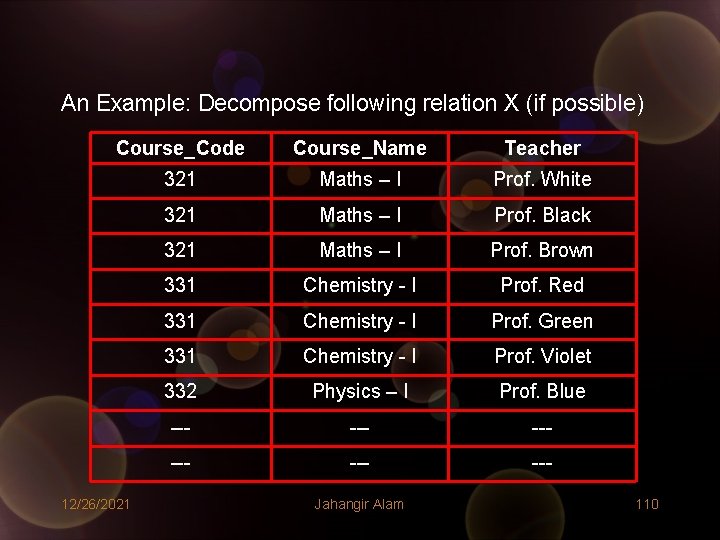
An Example: Decompose following relation X (if possible) Course_Code Course_Name Teacher 321 Maths – I Prof. White 321 Maths – I Prof. Black 321 Maths – I Prof. Brown 331 Chemistry - I Prof. Red 331 Chemistry - I Prof. Green 331 Chemistry - I Prof. Violet 332 Physics – I Prof. Blue --- --- --- 12/26/2021 Jahangir Alam 110

SOLUTION: • We can easily see that the following FD holds on the above relation: FD: X. Course_Code X. Course_Name Applying Heath’s theorem the given relation may be non-lossly decomposed as: X 1 <Course_Code, Course_Name> X 2<Course_Code, Teacher> Course_Code Course_Name Course_Code Teacher 321 Maths - I 321 Prof. White 331 Chemistry-I 321 Prof. Black 332 Physics - I 321 Prof. Brown --- --- --- 12/26/2021 Jahangir Alam 111

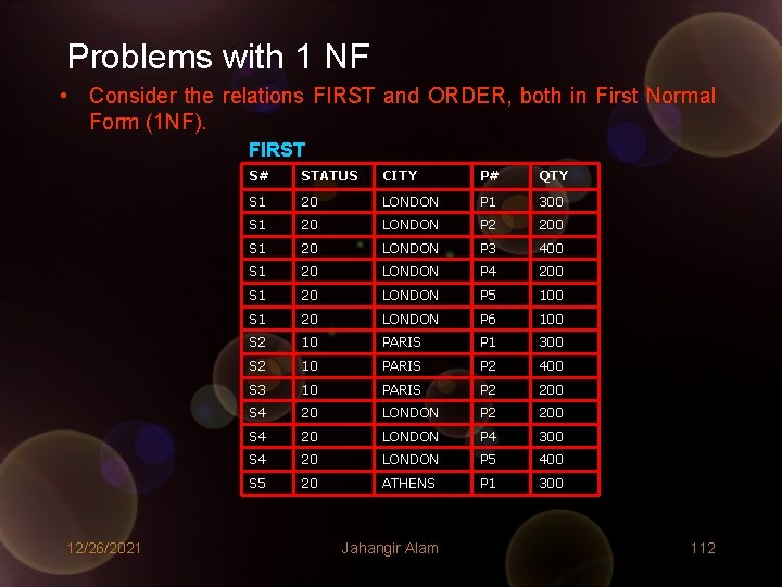
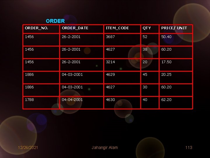
Problems with 1 NF • Consider the relations FIRST and ORDER, both in First Normal Form (1 NF). FIRST 12/26/2021 S# STATUS CITY P# QTY S 1 20 LONDON P 1 300 S 1 20 LONDON P 2 200 S 1 20 LONDON P 3 400 S 1 20 LONDON P 4 200 S 1 20 LONDON P 5 100 S 1 20 LONDON P 6 100 S 2 10 PARIS P 1 300 S 2 10 PARIS P 2 400 S 3 10 PARIS P 2 200 S 4 20 LONDON P 4 300 S 4 20 LONDON P 5 400 S 5 20 ATHENS P 1 300 Jahangir Alam 112

ORDER_NO. ORDER_DATE ITEM_CODE QTY PRICE/ UNIT 1456 26 -2 -2001 3687 52 50. 40 1456 26 -2 -2001 4627 38 60. 20 1456 26 -2 -2001 3214 20 17. 50 1886 04 -03 -2001 4629 45 20. 25 1886 04 -03 -2001 4627 30 60. 20 1788 04 -04 -2001 4630 40 62. 20 12/26/2021 Jahangir Alam 113

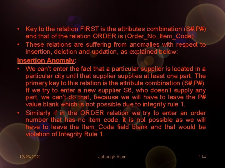
• Key to the relation FIRST is the attributes combination (S#, P#) and that of the relation ORDER is (Order_No. , Item_Code). • These relations are suffering from anomalies with respect to insertion, deletion and updation, as explained below: Insertion Anomaly: • We can’t enter the fact that a particular supplier is located in a particular city until that supplier supplies at least one part. The primary key to this relation is the attribute combination (S#, P#). If we try to enter a new supplier S 6, who doesn’t supply any part, we can’t do that, because we will have to leave the P# value blank which is not possible due to integrity rule 1. • Similarly if in the ORDER relation we try to enter an order number that has no item code, it is not possible as we will have to leave the Item_Code field blank and that would be violation of Integrity Rule 1. 12/26/2021 Jahangir Alam 114

Deletion Anomaly: • From the relation FIRST if we delete the supplier, having S#=‘S 5’, we not only destroy the shipment connecting to S 5, but also loose the information that S 5 is located in the city ATHENS. • Similarly, in the ORDER relation, if we delete the order for Order_No. =‘ 1788’, we loose the information that Price/ Unit for Item_code=‘ 4630’ is Rs. 62. 20. Updation Anomaly: • If the supplier S 1 changes its city from LONDON to ATHENS, then it is required to update several tuples for STATUS and CITY. This may lead to inconsistent values in the table. • Similarly, in ORDER relation if the price for Item_code 4627 cahnges to 63. 75, then we have to modify several tuples resulting more chances of inconstancies. 12/26/2021 Jahangir Alam 115

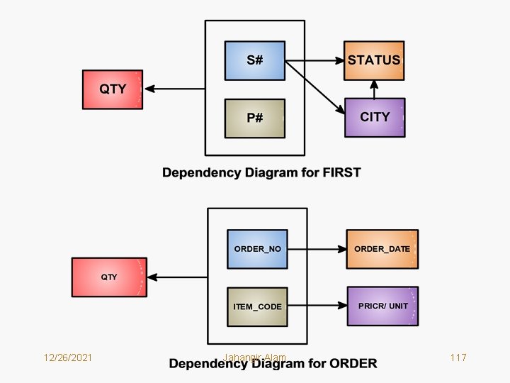
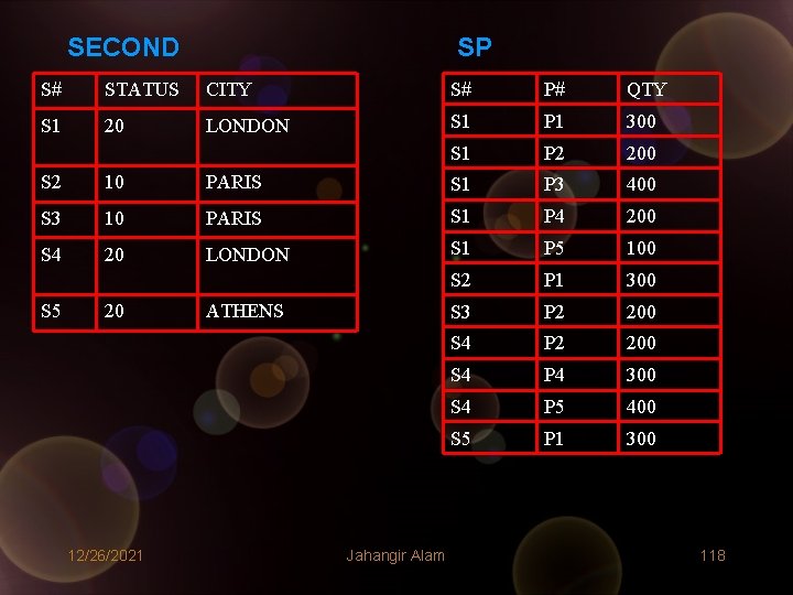
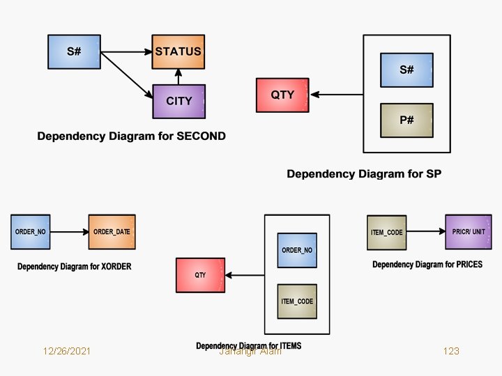
• To solve these problems what we should do? • First we draw the dependency diagrams for these relations. They have been shown on the next page. • Now, we decompose these relation as follows: Decomposition of FIRST: SECOND<S#, STATUS, CITY> SP<S#, P#, QTY> Decomposition of ORDER: XORDER<ORDER_NO, ORDER_DATE> PRICES<ITEM_CODE, PRICE/UNIT> ITEMS<ORDER_NO, ITEM_CODE, QTY> • Related tables show the instances of new relations. 12/26/2021 Jahangir Alam 116

12/26/2021 Jahangir Alam 117

SECOND SP S# STATUS CITY S# P# QTY S 1 20 LONDON S 1 P 1 300 S 1 P 2 200 S 2 10 PARIS S 1 P 3 400 S 3 10 PARIS S 1 P 4 200 S 4 20 LONDON S 1 P 5 100 S 2 P 1 300 S 3 P 2 200 S 4 P 4 300 S 4 P 5 400 S 5 P 1 300 S 5 20 12/26/2021 ATHENS Jahangir Alam 118

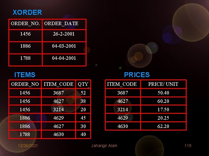
XORDER_NO. ORDER_DATE 1456 26 -2 -2001 1886 04 -03 -2001 1788 04 -04 -2001 ITEMS PRICES ORDER_NO ITEM_CODE QTY ITEM_CODE PRICE/ UNIT 1456 3687 52 3687 50. 40 1456 4627 38 4627 60. 20 1456 3214 20 3214 17. 50 1886 4629 45 4629 20. 25 1886 4627 30 4630 62. 20 1788 4630 40 12/26/2021 Jahangir Alam 119

• With these decompositions now we shall observe how the insertion, deletion and updation anomalies problems related to 1 NF representations of these relations are solved: Insertion Anomaly: • We can now enter the information that S 6 is located in Washington, in spite of the fact that currently he doesn’t supply any part. • Similarly an order without any item description can be placed. Deletion Anomaly: • We can now delete the shipment connecting S 5 to P 2 and S 3 to P 2 by deleting appropriate tuples from the relation SP, yet we don’t loose the information that they are located in which particular cities. • Similarly, if an order is cancelled we can delete appropriate tuple from XORDER relation and this time we don’t loose the price of the item (s) described in that order. 12/26/2021 Jahangir Alam 120

Updation Anomaly: • In the revised structures of the relations, the CITY of a given supplier appears once, so if a supplier moves from one city to another, his location can easily be altered. • Similarly the PRICE/ UNIT of an item can be changed easily in the PRICES relation. 12/26/2021 Jahangir Alam 121

What We Have Actually Done to Solve The Problems? ? • We have decomposed the relations in such a way that in each of the resultant relations every non key attribute is fully functionally dependent on the key attribute. • Check the dependency diagrams of new relations below: 12/26/2021 Jahangir Alam 122

12/26/2021 Jahangir Alam 123

Second Normal Form (2 NF) • A relation R is in Second Normal Form (2 NF) if and only if it is in First Normal Form (1 NF) and every non key attribute is fully functionally dependent on the key attribute. • Further a relational schema is said to be in 2 NF if each relation in the schema is in 2 NF. 12/26/2021 Jahangir Alam 124

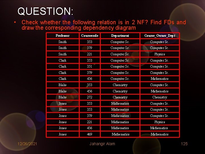
QUESTION: • Check whether the following relation is in 2 NF? Find FDs and draw the corresponding dependency diagram 12/26/2021 Professor Coursecode Department Course_Owner_Dept Smith 353 Computer Sc. Smith 379 Computer Sc. Smith 221 Computer Sc. Physics Clark 353 Computer Sc. Clark 351 Computer Sc. Clark 379 Computer Sc. Clark 456 Computer Sc. Mathematics Blake 353 Chemistry Computer Sc. Blake 456 Chemistry Mathematics Blake 272 Chemistry Jones 353 Mathematics Computer Sc. Jones 379 Mathematics Computer Sc. Jones 221 Mathematics Physics Jones 456 Mathematics Jones 469 Mathematics Jahangir Alam 125

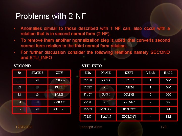
Problems with 2 NF • • • Anomalies similar to those described with 1 NF can, also occur with a relation that is in second normal form (2 NF). To remove them another normalization step is used, that converts second normal form relation to the third normal form relation. For further discussion consider the following relations namely SECOND and STU_INFO SECOND STU_INFO S# STATUS CITY ENo. NAME DEPT YEAR HALL S 1 20 LONDON Y-100 RAMA PHYSICS 1 MM S 2 10 PARIS Y-212 ALI CHEM 1 MM S 3 10 PARIS Y-107 RAVI MATHS 2 MM S 4 20 LONDON Z-551 TONI BOTANY 2 MM S 5 20 ATHENS X-553 MOHAN GEOLOGY 3 AI T-337 RAJAN ZOOLOGY 4 RM 12/26/2021 Jahangir Alam 126

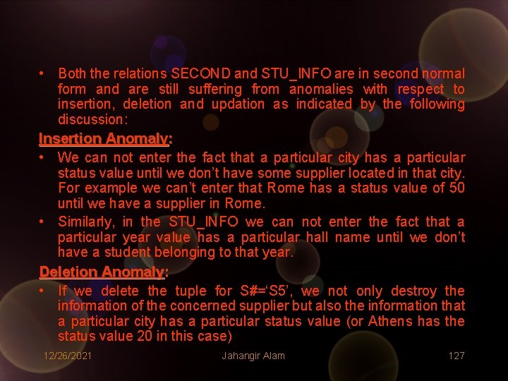
• Both the relations SECOND and STU_INFO are in second normal form and are still suffering from anomalies with respect to insertion, deletion and updation as indicated by the following discussion: Insertion Anomaly: • We can not enter the fact that a particular city has a particular status value until we don’t have some supplier located in that city. For example we can’t enter that Rome has a status value of 50 until we have a supplier in Rome. • Similarly, in the STU_INFO we can not enter the fact that a particular year value has a particular hall name until we don’t have a student belonging to that year. Deletion Anomaly: • If we delete the tuple for S#=‘S 5’, we not only destroy the information of the concerned supplier but also the information that a particular city has a particular status value (or Athens has the status value 20 in this case) 12/26/2021 Jahangir Alam 127

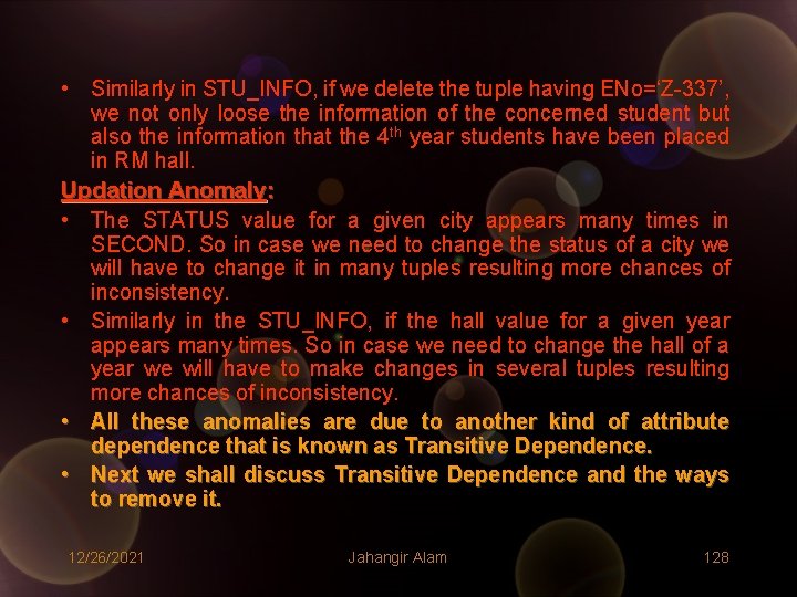
• Similarly in STU_INFO, if we delete the tuple having ENo=‘Z-337’, we not only loose the information of the concerned student but also the information that the 4 th year students have been placed in RM hall. Updation Anomaly: • The STATUS value for a given city appears many times in SECOND. So in case we need to change the status of a city we will have to change it in many tuples resulting more chances of inconsistency. • Similarly in the STU_INFO, if the hall value for a given year appears many times. So in case we need to change the hall of a year we will have to make changes in several tuples resulting more chances of inconsistency. • All these anomalies are due to another kind of attribute dependence that is known as Transitive Dependence. • Next we shall discuss Transitive Dependence and the ways to remove it. 12/26/2021 Jahangir Alam 128

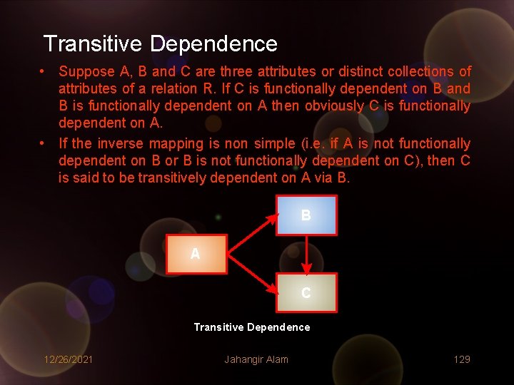
Transitive Dependence • Suppose A, B and C are three attributes or distinct collections of attributes of a relation R. If C is functionally dependent on B and B is functionally dependent on A then obviously C is functionally dependent on A. • If the inverse mapping is non simple (i. e. if A is not functionally dependent on B or B is not functionally dependent on C), then C is said to be transitively dependent on A via B. B A C Transitive Dependence 12/26/2021 Jahangir Alam 129

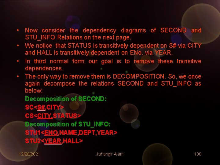
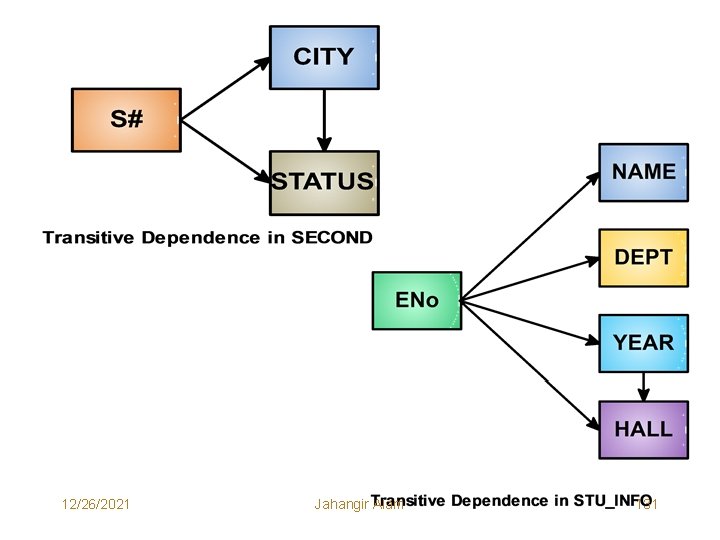
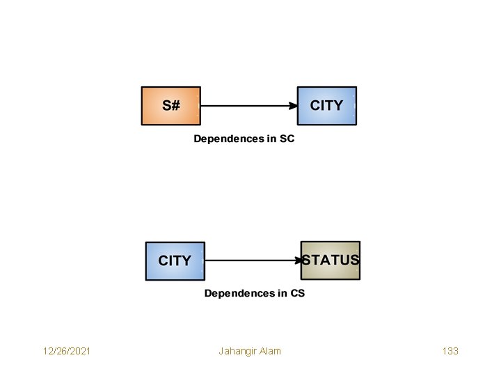
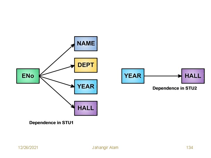
• Now consider the dependency diagrams of SECOND and STU_INFO Relations on the next page. • We notice that STATUS is transitively dependent on S# via CITY and HALL is transitively dependent on ENo. via YEAR. • In third normal form our goal is to remove these transitive dependences. • The only way to remove them is DECOMPOSITION. So, we once again decompose the relations SECOND and STU_INFO as below: Decomposition of SECOND: SC<S#, CITY> CS<CITY, STATUS> Decomposition of STU_INFO: STU 1<ENO, NAME, DEPT, YEAR> STU 2<YEAR, HALL> 12/26/2021 Jahangir Alam 130

12/26/2021 Jahangir Alam 131

Third Normal Form • A Relation R is said to be in third normal form (3 NF) if and only if it is in second normal form (2 NF) and every non-key attribute is nontransitively dependent on the primary key (key attribute). • A relational schema is in 3 NF if all of its relations are in 3 NF. • Consider the dependency diagrams (on next pages) for the relations SC, CS, STU 1 and STU 2 and note that all of them are in 3 NF. 12/26/2021 Jahangir Alam 132

12/26/2021 Jahangir Alam 133

12/26/2021 Jahangir Alam 134

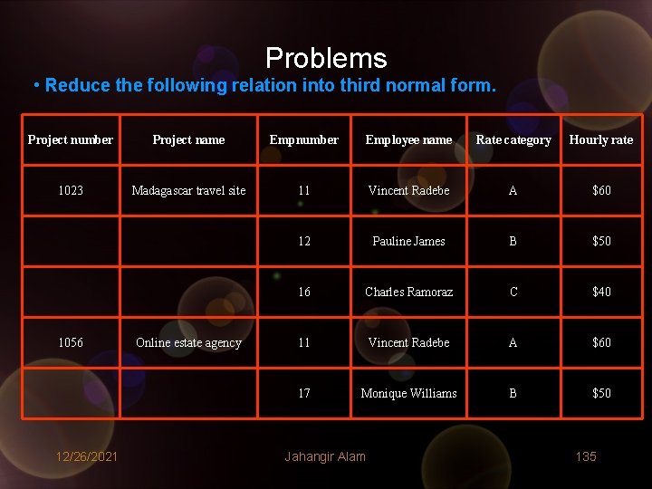
Problems • Reduce the following relation into third normal form. Project number Project name Empnumber Employee name Rate category Hourly rate 1023 Madagascar travel site 11 Vincent Radebe A $60 12 Pauline James B $50 16 Charles Ramoraz C $40 11 Vincent Radebe A $60 17 Monique Williams B $50 1056 12/26/2021 Online estate agency Jahangir Alam 135

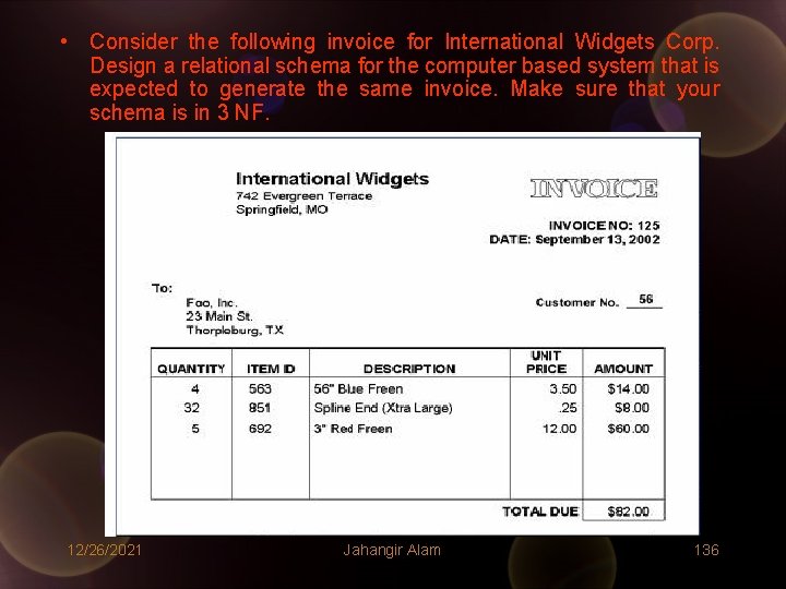
• Consider the following invoice for International Widgets Corp. Design a relational schema for the computer based system that is expected to generate the same invoice. Make sure that your schema is in 3 NF. 12/26/2021 Jahangir Alam 136

Relational Algebra & Relational Calculus Introduction • In 1971 E. F. Codd published two papers introducing the relational data model and relational data manipulation languages – Relational Algebra and Relational Calculus. • Both of these languages allow the manipulation of data solely on the basis of their logical characteristics. • In his original paper Codd introduced the relational data model and relational algebra. • Relational Algebra is a procedural language for manipulating relations i. e. relational algebra uses a step by step procedure to create a relation containing the data that answer the query. • In subsequent paper Codd introduced Relational Calculus. Relational calculus is non-procedural. In relational calculus a query is solved by defining a solution relation in a single step 12/26/2021 Jahangir Alam 137

• Codd showed that relational algebra and relational calculus are logically equivalent. It meant that any query that could be formulated in relational calculus could also be formulated in relational algebra and vice versa. • This provided a means of measuring logical power of a query language. If a language was at least as powerful as relational algebra or relational calculus, it was called Relationally Complete Language. • Thus, as commercial languages are developed their logical power can be tested by comparing them with relational algebra or relational calculus. If a language is less powerful than either of these, there will be certain queries which could not be formulated in that language. • Relational Algebra is important because it contributes much of the vocabulary and many of the basic relational data manipulation concepts that are used in commercial database languages. • Terms like selection, projection, join etc originate from relational algebra. 12/26/2021 Jahangir Alam 138

• Relational Calculus is important from following two reasons: – It is based on predicate calculus of formal logic, which is a powerful method of determining the truth of a statement from the truth of its components. – Several commercial relational languages (including SQL) are conceptually close to it. • Both relational algebra and relational calculus are theoretical languages, so here we are interested only in the conceptual aspects of algebra and calculus not in any specific implementations of them. 12/26/2021 Jahangir Alam 139

Relational Algebra • Relational Algebra operators manipulate relations i. e. these operators use one or two existing relations to create a new relation. This new relation may then be used as an input to a new operation. • This powerful concept i. e. the creation of new relations from old ones makes possible an infinite variety of data manipulations. It also makes the solution of queries easier, since we can experiment with partial solution until we find an approach that will lead us to the final solution. • The relational algebra operators can be divided into following two categories: – Basic Set Oriented Operations – Relational Oriented Operations 12/26/2021 Jahangir Alam 140

Basic Set Oriented Operations • These are traditional set operations namely Union, Difference, Intersection and Cartesian Product. • Three of these four basic operations – Union, Intersection and Difference require that operand relations must be union compatible which means that the names of the attributes of the operand relations are same and that the resultant relation inherits these names. Mathematically: • Two relations P and Q, are said to be union compatible if both P and Q are of same degree n and the domains of the corresponding n attributes are identical i. e. if P = {P 1, P 2, P 3, …. , Pn} and Q = {Q 1, Q 2, Q 3, …. , Qn} then: Dom(Pi) = Dom(Qi) for all i = 1 to n. Where Dom(Pi) represents the domain of the attribute Pi. • Next we discuss the basic set oriented operators of relational algebra. 12/26/2021 Jahangir Alam 141

1. Union (U) • If we assume that P and Q are two union compatible relations then the union of P and Q is set – theoretic union of P and Q. The resultant relation R = P U Q has tuples drawn from P and Q such that: R = { t | t є P V t є Q } and max(|P|, |Q|) ≤ |R| ≤ |P| + |Q| Note: |X| means cardinality of relation X. • Following example illustrates: 12/26/2021 Jahangir Alam 142

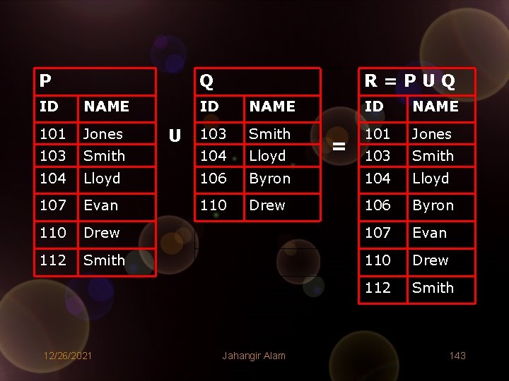
P Q ID NAME 101 Jones 103 R=PUQ ID NAME 103 Smith 101 Jones Smith 104 Lloyd 103 Smith 104 Lloyd 106 Byron 104 Lloyd 107 Evan 110 Drew 106 Byron 110 Drew 107 Evan 112 Smith 110 Drew 112 Smith 12/26/2021 U Jahangir Alam = 143

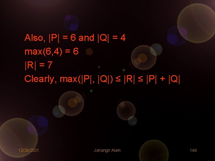
Also, |P| = 6 and |Q| = 4 max(6, 4) = 6 |R| = 7 Clearly, max(|P|, |Q|) ≤ |R| ≤ |P| + |Q| 12/26/2021 Jahangir Alam 144

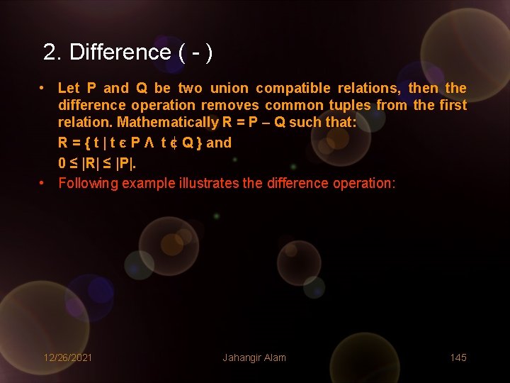
2. Difference ( - ) • Let P and Q be two union compatible relations, then the difference operation removes common tuples from the first relation. Mathematically R = P – Q such that: R = { t | t є P Λ t є Q } and 0 ≤ |R| ≤ |P|. • Following example illustrates the difference operation: 12/26/2021 Jahangir Alam 145

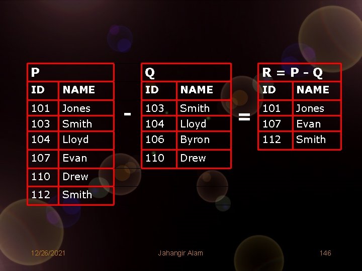
P Q ID NAME 101 Jones 103 Smith 104 R=P-Q ID NAME 103 Smith 101 Jones 104 Lloyd 107 Evan Lloyd 106 Byron 112 Smith 107 Evan 110 Drew 112 Smith 12/26/2021 - Jahangir Alam = 146

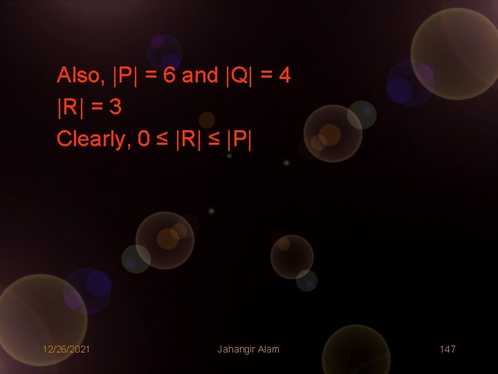
Also, |P| = 6 and |Q| = 4 |R| = 3 Clearly, 0 ≤ |R| ≤ |P| 12/26/2021 Jahangir Alam 147

3. Intersection (∩) • If we assume that P and Q are two union compatible relations then intersection operation selects the common tuples from P and Q. The resultant relation R = P ∩ Q has tuples drawn from P and Q such that: R = { t | t є P Λ t є Q } and 0 ≤ |R| ≤ min(|P|, |Q|) Note: |X| means cardinality of relation X. • Following example illustrates the intersection operation: 12/26/2021 Jahangir Alam 148

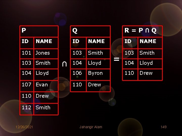
P ID Q NAME R=P∩Q ID NAME 101 Jones 103 Smith 104 Lloyd 106 Byron 110 Drew 107 Evan 110 Drew ∩ = 110 Drew 112 Smith 12/26/2021 Jahangir Alam 149

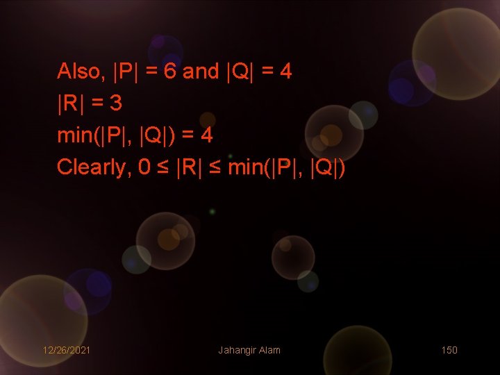
Also, |P| = 6 and |Q| = 4 |R| = 3 min(|P|, |Q|) = 4 Clearly, 0 ≤ |R| ≤ min(|P|, |Q|) 12/26/2021 Jahangir Alam 150

4. Cartesian Product (X) • The Extended Cartesian product or simply the Cartesian Product of two relations is the concatenation of tuples belonging to the two relations. • A new resultant relation is created, consisting of all possible combination of tuples. Mathematically: R = P X Q = { t 1 || t 2 | t 1 є P Λ t 2 є Q } • The degree of the resultant relation is given by: Deg(R) = Deg(P) + Deg(Q) • The cardinality of resultant relation is given by: |R| = |P| * |Q| 12/26/2021 Jahangir Alam 151

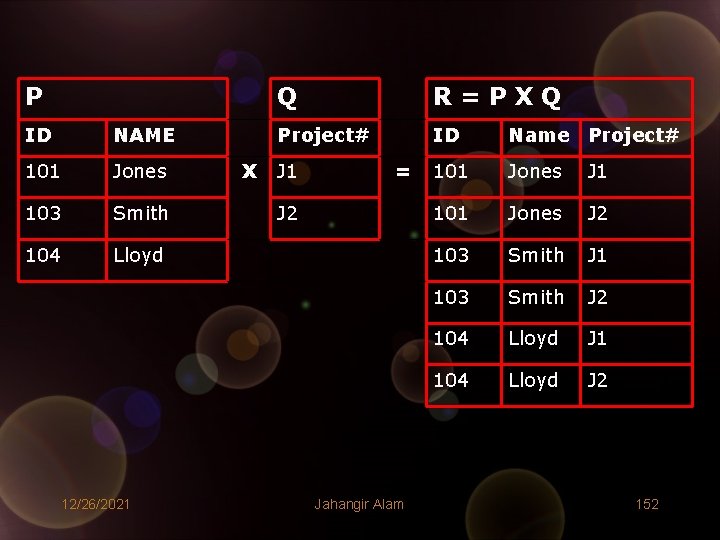
P ID NAME 101 Jones 103 Smith 104 Lloyd 12/26/2021 X Q R=PXQ Project# ID Name Project# 101 Jones J 1 101 Jones J 2 103 Smith J 1 103 Smith J 2 104 Lloyd J 1 104 Lloyd J 2 J 1 = J 2 Jahangir Alam 152

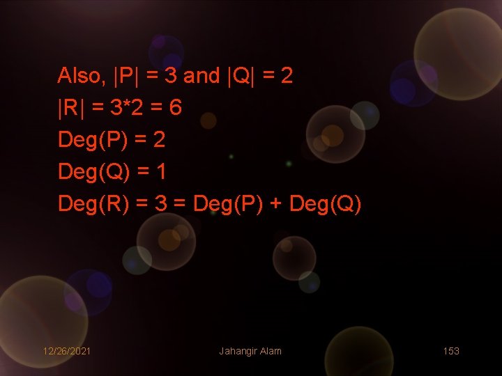
Also, |P| = 3 and |Q| = 2 |R| = 3*2 = 6 Deg(P) = 2 Deg(Q) = 1 Deg(R) = 3 = Deg(P) + Deg(Q) 12/26/2021 Jahangir Alam 153

Relational Oriented Operations • They are also known as Additional Relational Algebra Operations. • The Basic Set Operations which have very limited data manipulation capabilities have been supplemented by the following additional operations: – – Projection (π) Selection (σ) Join ( ) Division (÷) • Projection and selection are unary operators (i. e. they require single operand) however Join and Division are binary operators. 12/26/2021 Jahangir Alam 154

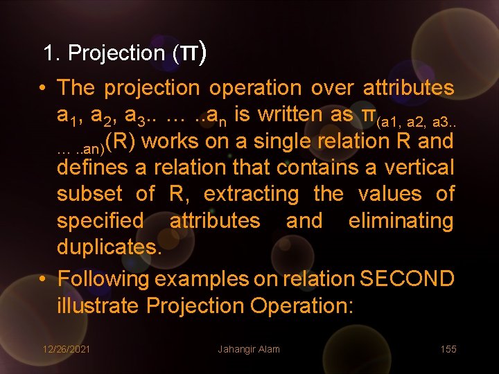
1. Projection (π) • The projection operation over attributes a 1, a 2, a 3. . …. . an is written as π(a 1, a 2, a 3. . …. . an)(R) works on a single relation R and defines a relation that contains a vertical subset of R, extracting the values of specified attributes and eliminating duplicates. • Following examples on relation SECOND illustrate Projection Operation: 12/26/2021 Jahangir Alam 155

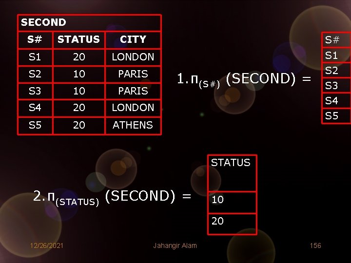
SECOND S# STATUS CITY S# S 1 20 LONDON S 1 S 2 10 PARIS S 2 S 3 10 PARIS S 4 20 LONDON S 5 20 ATHENS 1. π(S#) (SECOND) = S 4 S 5 STATUS 2. π(STATUS) (SECOND) = 10 20 12/26/2021 Jahangir Alam S 3 156

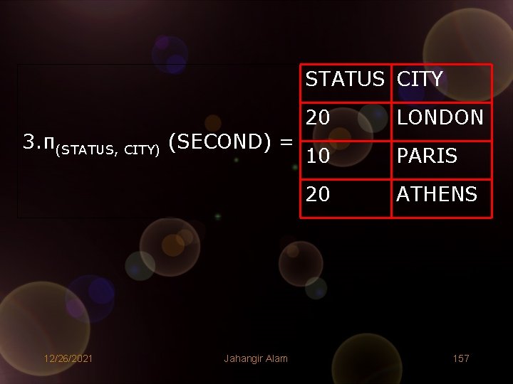
STATUS CITY 3. π(STATUS, CITY) (SECOND) = 12/26/2021 Jahangir Alam 20 LONDON 10 PARIS 20 ATHENS 157

2. Selection Operation (σ) • The selection operation written as σpredicate(R), works on a single relation R and defines a relation that contains only those tuples of R that satisfy the specified condition (predicate) for a given attribute or for a combination of attributes. • Following examples on relations P and SECOND illustrate the Selection operation. 12/26/2021 Jahangir Alam 158

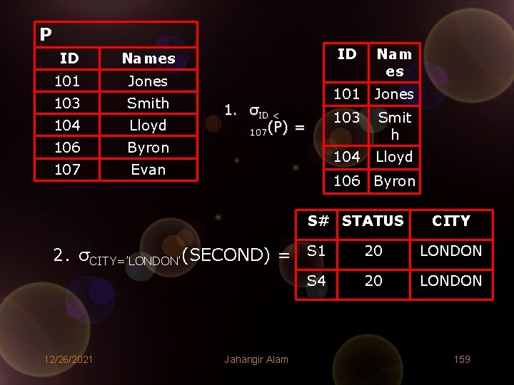
P ID Names 101 Jones 103 Smith 104 Lloyd 106 Byron 107 Evan 1. σID < 107(P) = ID Nam es 101 Jones 103 Smit h 104 Lloyd 106 Byron S# STATUS CITY 2. σCITY=’LONDON’(SECOND) = S 1 20 LONDON S 4 20 LONDON 12/26/2021 Jahangir Alam 159

• Write Relational Algebra expression to answer the following query for relation SECOND: “Get S# for all suppliers residing in PARIS”. • Solution: 1. Select all suppliers residing in Paris: σCITY=’PARIS’(SECOND) 2. Project Out the undesired attributes (or take projection on S#) π(S#) (σCITY=’PARIS’(SECOND)) 12/26/2021 Jahangir Alam 160

3. Join ( ) • The Join operation as its name suggests, allows the combination of two relations to form a single new relation. The join operation is used to connect data across relations, which is the most important function in any database language. • There are several versions of join namely: – – – Natural Join Theta Join Equi Join Self Join Outer Join • Join is supposed to be one of the most important operations of relational databases. 12/26/2021 Jahangir Alam 161

(i) Natural Join • Suppose we want to take Natural Join of two relations P and Q which have columns C 1, C 2, C 3…. …. …. Cn in common. Then, P Q is obtained as: 1. Take Cartesian Product of P and Q i. e. Find P X Q. 2. Eliminate all tuples from P X Q except those on which the values of columns C 1, C 2, C 3…. …. …. Cn, in P are equal, respectively to the values of those columns in Q. 3. Project out one copy of the columns C 1, C 2, C 3…. …. …. Cn. • • The degree of resultant relation is always less than the sum of the degree of P and degree of Q. Following example illustrates the Natural Join operation: 12/26/2021 Jahangir Alam 162

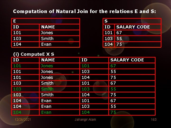
Computation of Natural Join for the relations E and S: E ID 101 103 104 NAME Jones Smith Evan (i) Compute. E X S ID NAME 101 Jones 103 Smith 104 Evan 12/26/2021 S ID 101 103 104 Jahangir Alam SALARY CODE 67 55 75 163

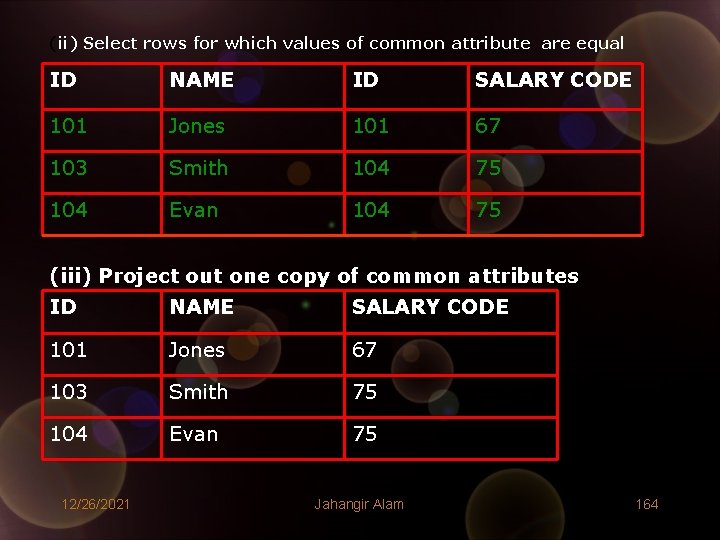
(ii) Select rows for which values of common attribute are equal ID NAME ID SALARY CODE 101 Jones 101 67 103 Smith 104 75 104 Evan 104 75 (iii) Project out one copy of common attributes ID NAME SALARY CODE 101 Jones 67 103 Smith 75 104 Evan 75 12/26/2021 Jahangir Alam 164

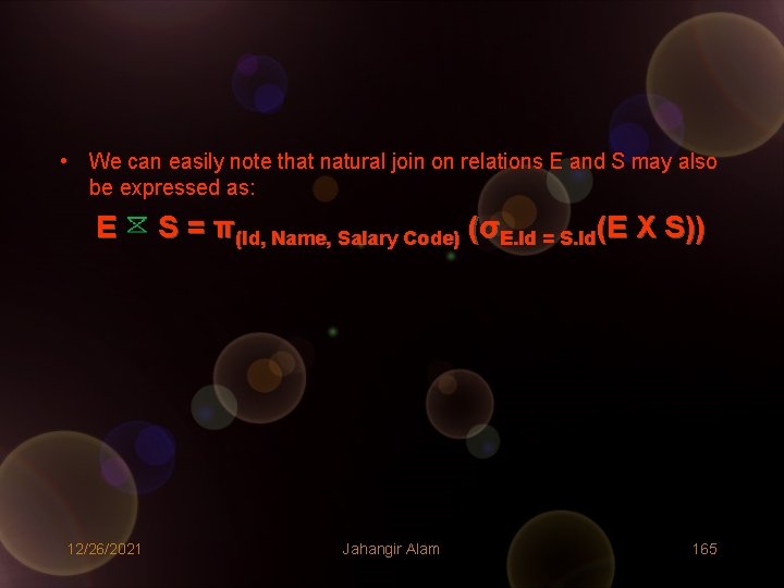
• We can easily note that natural join on relations E and S may also be expressed as: E 12/26/2021 S = π(Id, Name, Salary Code) (σE. Id = S. Id(E X S)) Jahangir Alam 165

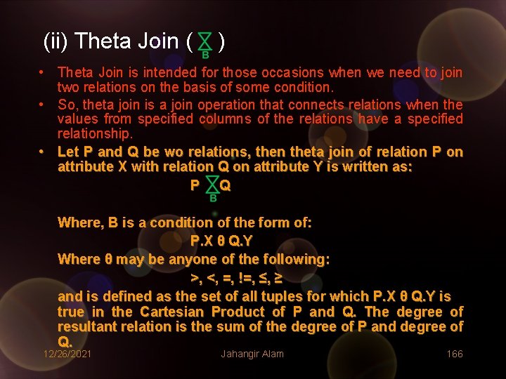
(ii) Theta Join ( ) • Theta Join is intended for those occasions when we need to join two relations on the basis of some condition. • So, theta join is a join operation that connects relations when the values from specified columns of the relations have a specified relationship. • Let P and Q be wo relations, then theta join of relation P on attribute X with relation Q on attribute Y is written as: P Q Where, B is a condition of the form of: P. X θ Q. Y Where θ may be anyone of the following: >, <, =, !=, ≤, ≥ and is defined as the set of all tuples for which P. X θ Q. Y is true in the Cartesian Product of P and Q. The degree of resultant relation is the sum of the degree of P and degree of Q. 12/26/2021 Jahangir Alam 166

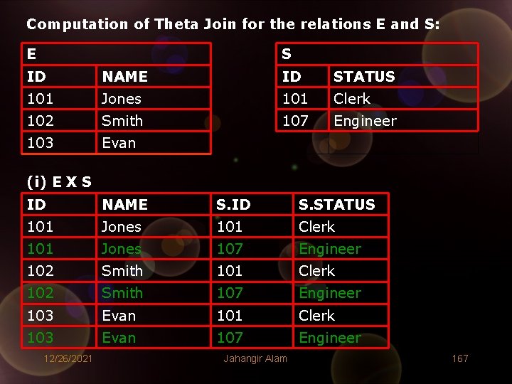
Computation of Theta Join for the relations E and S: E S ID NAME ID STATUS 101 Jones 101 Clerk 102 Smith 107 Engineer 103 Evan (i) E X S ID NAME S. ID S. STATUS 101 Jones 101 Clerk 101 Jones 107 Engineer 102 Smith 101 Clerk 102 Smith 107 Engineer 103 Evan 101 Clerk 103 Evan 107 Engineer 12/26/2021 Jahangir Alam 167

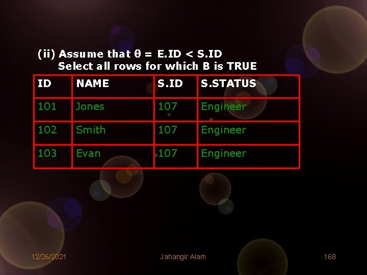
(ii) Assume that θ = E. ID < S. ID Select all rows for which B is TRUE ID NAME S. ID S. STATUS 101 Jones 107 Engineer 102 Smith 107 Engineer 103 Evan 107 Engineer 12/26/2021 Jahangir Alam 168

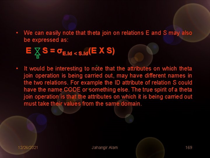
• We can easily note that theta join on relations E and S may also be expressed as: E S = σE. Id < S. Id(E X S) • It would be interesting to note that the attributes on which theta join operation is being carried out, may have different names in the two relations. For example the ID attribute of relation S could have the name CODE or something else. The true spirit of a theta join operation is that the attributes on which it is being carried out must take their values from the same domain. 12/26/2021 Jahangir Alam 169

(iii) Equi Join: • Theta join is called Equi Join when the condition for comparison (θ) is equality. • Clearly, Equi Join is a special case of Theta Join. • Also, Natural Join is a special case of Equi Join where, among the duplicate copies of columns, one copy is projected out. • One major distinction between Equi Join and Natural Join is that, for Natural Join it is mandatory that the attributes on which natural join operation is being carried out must have same names in the two relations however in case of equi join they may have different names. • Following example illustrates EQUI Join: 12/26/2021 Jahangir Alam 170

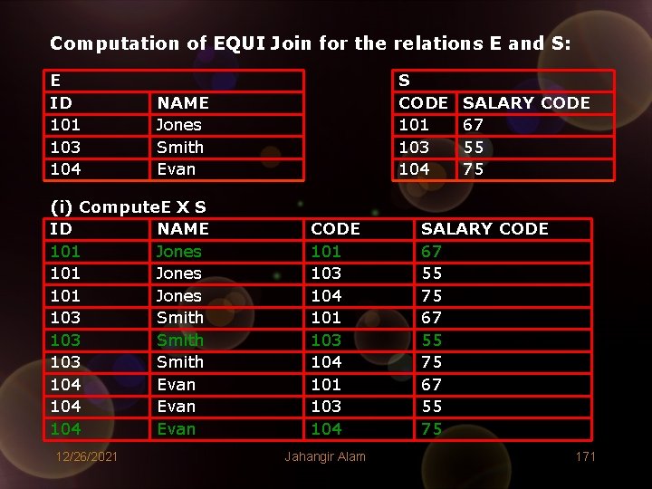
Computation of EQUI Join for the relations E and S: E ID 101 103 104 NAME Jones Smith Evan (i) Compute. E X S ID NAME 101 Jones 103 Smith 104 Evan 12/26/2021 S CODE 101 103 104 Jahangir Alam SALARY CODE 67 55 75 171

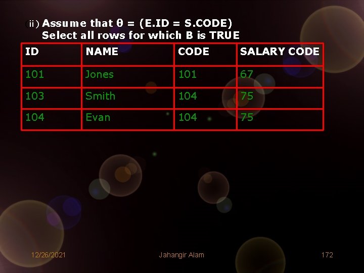
(ii) Assume that θ = (E. ID = S. CODE) Select all rows for which B is TRUE ID NAME CODE SALARY CODE 101 Jones 101 67 103 Smith 104 75 104 Evan 104 75 12/26/2021 Jahangir Alam 172

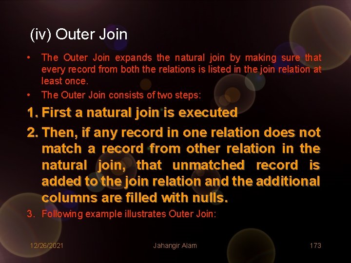
(iv) Outer Join • • The Outer Join expands the natural join by making sure that every record from both the relations is listed in the join relation at least once. The Outer Join consists of two steps: 1. First a natural join is executed 2. Then, if any record in one relation does not match a record from other relation in the natural join, that unmatched record is added to the join relation and the additional columns are filled with nulls. 3. Following example illustrates Outer Join: 12/26/2021 Jahangir Alam 173

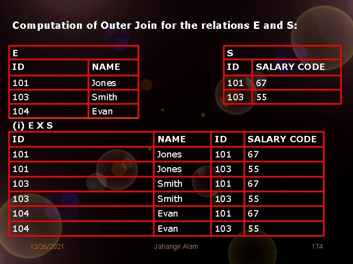
Computation of Outer Join for the relations E and S: E S ID NAME ID SALARY CODE 101 Jones 101 67 103 Smith 103 55 104 Evan (i) E X S ID NAME ID SALARY CODE 101 Jones 101 67 101 Jones 103 55 103 Smith 101 67 103 Smith 103 55 104 Evan 101 67 104 Evan 103 55 12/26/2021 Jahangir Alam 174

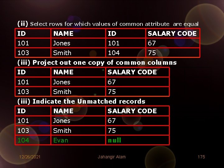
(ii) Select rows for which values of common attribute are equal ID NAME ID SALARY CODE 101 Jones 101 67 103 Smith 104 75 (iii) Project out one copy of common columns ID NAME SALARY CODE 101 Jones 67 103 Smith 75 (iii) Indicate the Unmatched records ID NAME SALARY CODE 101 Jones 67 103 Smith 75 104 Evan null 12/26/2021 Jahangir Alam 175

Please Note… • Strictly speaking the outer join operation we have just executed is a Left Outer Join as it keeps every tuple in the left hand relation in the result. • Similarly there is a Right Outer Join, that keeps every tuple in the right hand relation in the result. • There is also a Full Outer Join that keeps all tuples in both relations, padding tuples with nulls when no matching tuples are found. 12/26/2021 Jahangir Alam 176

(v) Self Join • As the name indicates, self join means joining a relation with itself. • But how to join a relation with itself when all the attributes are common and take the values from identical domains. • To resolve the problem we copy the relation into another relation having a different name and join operation is executed on the qualified attributes indicated by the requirement i. e. by the query. • Following example illustrates: 12/26/2021 Jahangir Alam 177

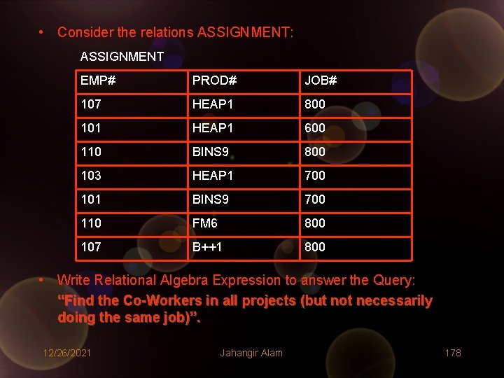
• Consider the relations ASSIGNMENT: ASSIGNMENT EMP# PROD# JOB# 107 HEAP 1 800 101 HEAP 1 600 110 BINS 9 800 103 HEAP 1 700 101 BINS 9 700 110 FM 6 800 107 B++1 800 • Write Relational Algebra Expression to answer the Query: “Find the Co-Workers in all projects (but not necessarily doing the same job)”. 12/26/2021 Jahangir Alam 178

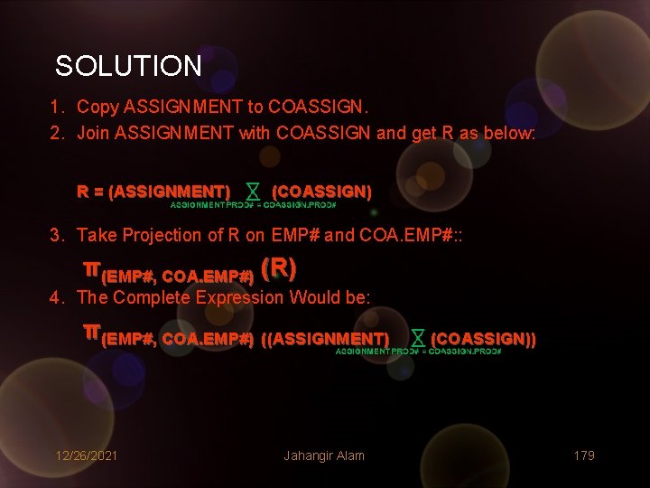
SOLUTION 1. Copy ASSIGNMENT to COASSIGN. 2. Join ASSIGNMENT with COASSIGN and get R as below: R = (ASSIGNMENT) (COASSIGN) 3. Take Projection of R on EMP# and COA. EMP#: : π(EMP#, COA. EMP#) (R) 4. The Complete Expression Would be: π(EMP#, COA. EMP#) ((ASSIGNMENT) 12/26/2021 Jahangir Alam (COASSIGN)) 179

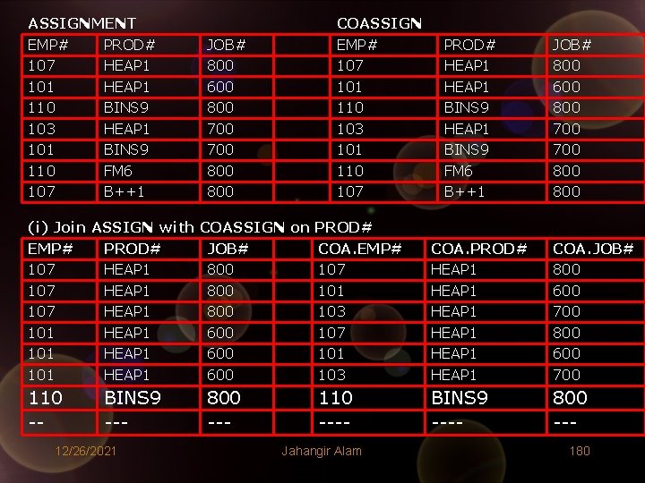
ASSIGNMENT EMP# PROD# 107 HEAP 1 101 HEAP 1 110 BINS 9 103 HEAP 1 101 BINS 9 110 FM 6 107 B++1 (i) Join ASSIGN with EMP# PROD# 107 HEAP 1 101 HEAP 1 110 -- BINS 9 --- 12/26/2021 JOB# 800 600 800 700 800 COASSIGN EMP# 107 101 110 103 101 110 107 COASSIGN on PROD# JOB# COA. EMP# 800 107 800 101 800 103 600 107 600 101 600 103 800 --- 110 ---Jahangir Alam PROD# HEAP 1 BINS 9 FM 6 B++1 JOB# 800 600 800 700 800 COA. PROD# HEAP 1 HEAP 1 COA. JOB# 800 600 700 BINS 9 ---- 800 --180

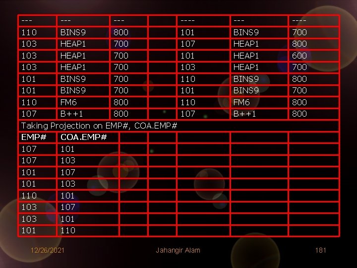
------110 BINS 9 800 103 HEAP 1 700 101 BINS 9 700 110 FM 6 800 107 B++1 800 Taking Projection on EMP#, COA. EMP# 107 101 107 103 101 107 101 103 110 101 103 107 103 101 110 12/26/2021 ---101 107 101 103 110 101 110 107 Jahangir Alam --BINS 9 HEAP 1 BINS 9 FM 6 B++1 ---700 800 600 700 800 800 181

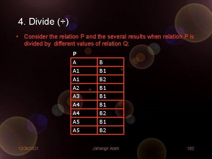
4. Divide (÷) • Consider the relation P and the several results when relation P is divided by different values of relation Q: P 12/26/2021 A B A 1 B 1 A 1 B 2 A 2 B 1 A 3 B 1 A 4 B 2 A 5 B 1 A 5 B 2 Jahangir Alam 182

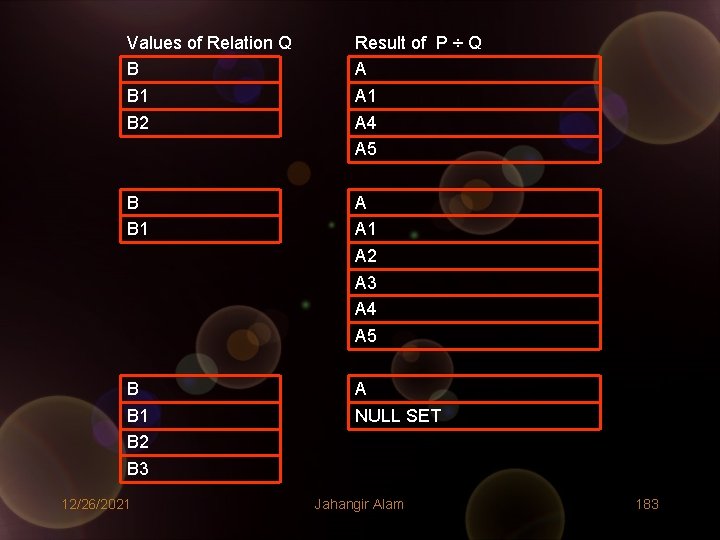
Values of Relation Q B B 1 B 2 Result of P ÷ Q A A 1 A 4 A 5 B B 1 A A 1 A 2 A 3 A 4 A 5 B B 1 B 2 B 3 A NULL SET 12/26/2021 Jahangir Alam 183

• Simply stated – The division of P and Q is defined such that the Cartesian Product of the result with Q is a subset of P. “OR” • If we assume that a tuple for an instance (A 1, B 1) of P represents the object A 1 with the property B 1 then resultant relation R is the set of all such instances from P that posses the property B 1. 12/26/2021 Jahangir Alam 184

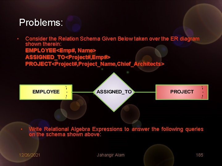
Problems: • Consider the Relation Schema Given Below taken over the ER diagram shown therein: EMPLOYEE<Emp#, Name> ASSIGNED_TO<Project#, Emp#> PROJECT<Project#, Project_Name, Chief_Architects> • Write Relational Algebra Expressions to answer the following queries on the schema shown above: 12/26/2021 Jahangir Alam 185

1. Get Emp# of employees working on project COMP 353. 2. Get details of employees (both number and name) working on project COMP 353. 3. Obtain details of employees working on Database projects. 4. Gather details of employees working on both COMP 353 and COMP 354. 5. Find the numbers of employees who work on at least all of the projects that employee 107 works on. 6. Find employee numbers of employees do not work on project COMP 453. 7. Get employee number of employees who work on all projects. 8. List the employee numbers of employees other than employee 107 who work on at least one project that employee 107 works on. 12/26/2021 Jahangir Alam 186

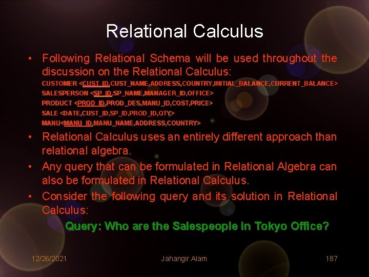
Relational Calculus • Following Relational Schema will be used throughout the discussion on the Relational Calculus: CUSTOMER <CUST_ID , CUST_NAME, ADDRESS, COUNTRY, INITIAL_BALANCE, CURRENT_BALANCE> <CUST_ID, CUST_NAME, ADDRESS, COUNTRY, INITIAL_BALANCE, CURRENT_BALANCE> SALESPERSON <SP_ID , SP_NAME, MANAGER_ID, OFFICE> <SP_ID, SP_NAME, MANAGER_ID, OFFICE> PRODUCT <PROD_ID , PROD_DES, MANU_ID, COST, PRICE> <PROD_ID, PROD_DES, MANU_ID, COST, PRICE> SALE <DATE, CUST_ID, SP_ID, PROD_ID, QTY> MANU<MANU_ID , MANU_NAME, ADDRESS, COUNTRY> MANU<MANU_ID, MANU_NAME, ADDRESS, COUNTRY> • Relational Calculus uses an entirely different approach than relational algebra. • Any query that can be formulated in Relational Algebra can also be formulated in Relational Calculus. • Consider the following query and its solution in Relational Calculus: Query: Who are the Salespeople in Tokyo Office? 12/26/2021 Jahangir Alam 187

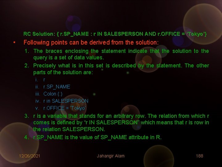
RC Solution: { r. SP_NAME : r IN SALESPERSON AND r. OFFICE = ‘Tokyo’} • Following points can be derived from the solution: 1. The braces enclosing the statement indicate that the solution to the query is a set of data values. 2. Precisely what is in this set is described by the statement. The other parts of the solution are: i. iii. iv. v. r r. SP_NAME Colon (: ) r in SALESPERSON r. OFFICE = ‘Tokyo’ 3. r is a variable that stands for an arbitrary row. The relation from which r comes is defined by “r IN SALESPERSON” which means that r is row in the relation SALESPERSON. 4. r. SP_NAME is the value of SP_NAME attribute in R. 12/26/2021 Jahangir Alam 188

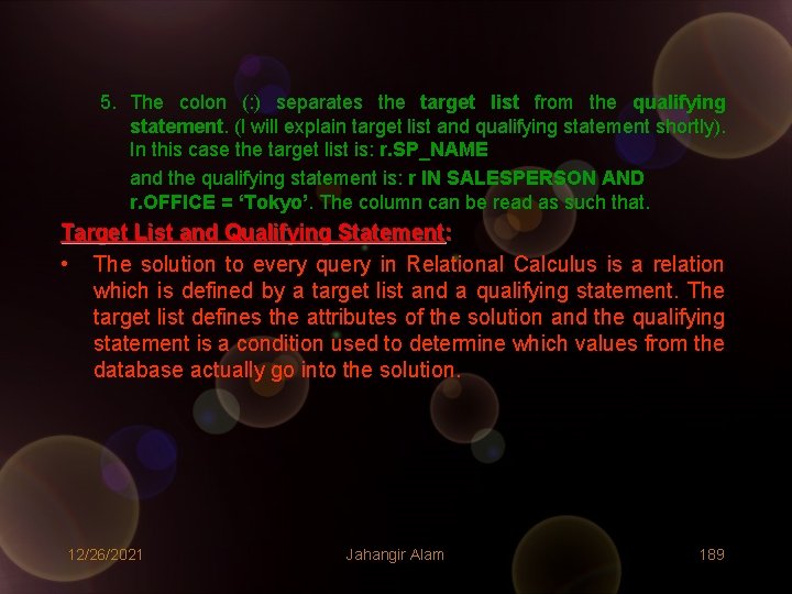
5. The colon (: ) separates the target list from the qualifying statement. (I will explain target list and qualifying statement shortly). In this case the target list is: r. SP_NAME and the qualifying statement is: r IN SALESPERSON AND r. OFFICE = ‘Tokyo’. The column can be read as such that. Target List and Qualifying Statement: • The solution to every query in Relational Calculus is a relation which is defined by a target list and a qualifying statement. The target list defines the attributes of the solution and the qualifying statement is a condition used to determine which values from the database actually go into the solution. 12/26/2021 Jahangir Alam 189

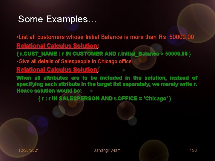
Some Examples… • List all customers whose Initial Balance is more than Rs. 50000. 00 Relational Calculus Solution: { r. CUST_NAME : r IN CUSTOMER AND r. Initial_Balance > 50000. 00 } • Give all details of Salespeople in Chicago office. Relational Calculus Solution: When all attributes are to be included in the solution, instead of specifying each attribute in the target list separately, we merely write r. Hence solution would be: { r : r IN SALESPERSON AND r. OFFICE = ‘Chicago’ } 12/26/2021 Jahangir Alam 190

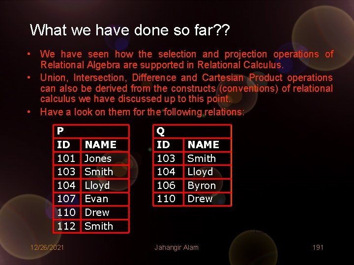
What we have done so far? ? • We have seen how the selection and projection operations of Relational Algebra are supported in Relational Calculus. • Union, Intersection, Difference and Cartesian Product operations can also be derived from the constructs (conventions) of relational calculus we have discussed up to this point. • Have a look on them for the following relations: P ID 101 103 104 107 110 112 12/26/2021 NAME Jones Smith Lloyd Evan Drew Smith Q ID 103 104 106 110 NAME Smith Lloyd Byron Drew Jahangir Alam 191

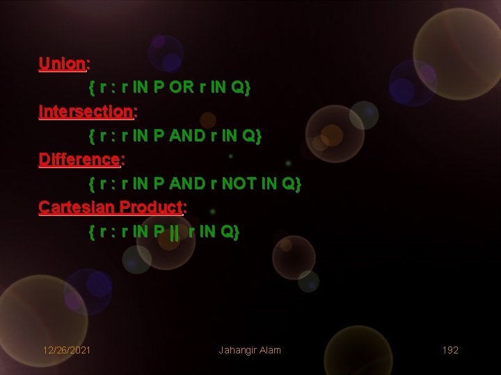
Union: { r : r IN P OR r IN Q} Intersection: { r : r IN P AND r IN Q} Difference: { r : r IN P AND r NOT IN Q} Cartesian Product: { r : r IN P || r IN Q} 12/26/2021 Jahangir Alam 192

What we have not done so far? ? • We have not shown the Relational Calculus equivalent for the following Relational Algebra operations: – Join (In Relational Calculus it requires use of Existential Qualifier) – Divide (In Relational Calculus it requires use of Universal Qualifier) Existential Qualifier and Join: • A qualifier qualifies or indicates the quality of something. • The existential qualifier states that at least one instance of a particular type of thing exists. • In Relational Calculus the existential qualifier is used to state that a particular type of row in a relation exists. • Consider the following query: “List Names of Customers who have purchased product 2518” 12/26/2021 Jahangir Alam 193

• Clearly, the solution to this query is a relation containing the names of certain customers. This is a single column relation so the target list is clearly – r. CUST_NAME. • What should be the qualifying statement? To be in the solution, the customer, must meet the condition of having purchased product 2518. In other words, if a given customer’s ID is found in a row of SALE with PROD_ID = 2518, then that customer is in the solution. • Thus the condition must be that there exists at least one row in SALE that contains the customer’s ID and a PROD_ID of 2518. We state it as follows: there exists s in SALE (s. CUST_ID = r. CUST_ID AND PROD_ID = ‘ 2518’) • This is read as “There exists a row in SALE, such that s. CUST_ID = r. CUST_ID AND PROD_ID = ‘ 2518’. (The words there exists constitute the existential qualifier. ) 12/26/2021 Jahangir Alam 194

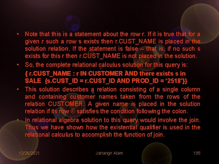
• Note that this is a statement about the row r. If it is true that for a given r such a row s exists then r. CUST_NAME is placed in the solution relation. If the statement is false – that is, if no such s exists for this r then r. CUST_NAME is not placed in the solution. • So, the complete relational calculus solution for this query is: { r. CUST_NAME : r IN CUSTOMER AND there exists s in SALE {s. CUST_ID = r. CUST_ID AND PROD_ID = ‘ 2518’}} • This solution describes a relation consisting of a single column and containing customer names taken from the rows of the relation CUSTOMER. A given name is placed in the solution relation if its row ® satisfies the condition following the colon. • In relational algebra solution to this query would involve the join. Thus we have shown how the existential qualifier is used in the relational calculus to accomplish the function of join. 12/26/2021 Jahangir Alam 195

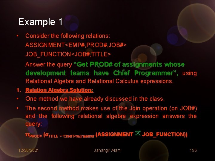
Example 1 • Consider the following relations: ASSIGNMENT<EMP#, PROD#, JOB#> JOB_FUNCTION<JOB#, TITLE> Answer the query “Get PROD# of assignments whose development teams have Chief Programmer”, using Relational Algebra and Relational Calculus expressions. 1. Relation Algebra Solution: • One method we have already discussed in the class. • The second method makes use of the Join operation (on JOB#) and the following relational algebra expression answers the query: πPROD# (σTITLE = ‘Chief Programmer’(ASSIGNMENT 12/26/2021 Jahangir Alam JOB_FUNCTION)) 196

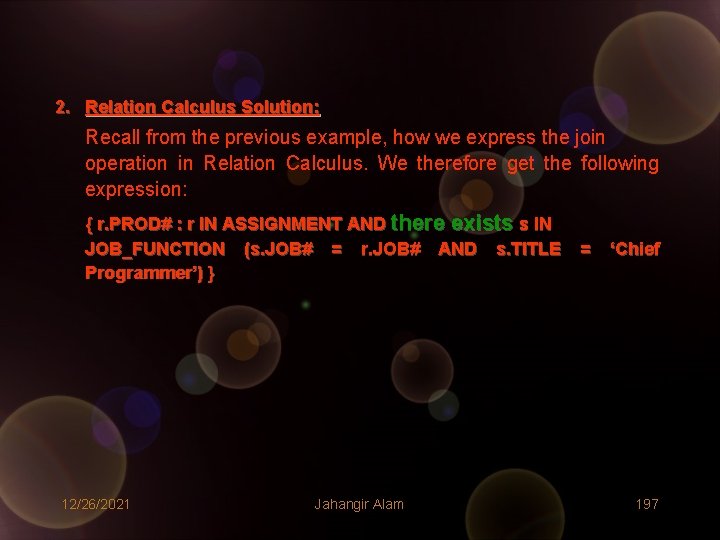
2. Relation Calculus Solution: Recall from the previous example, how we express the join operation in Relation Calculus. We therefore get the following expression: { r. PROD# : r IN ASSIGNMENT AND there exists s IN JOB_FUNCTION (s. JOB# = r. JOB# AND s. TITLE Programmer’) } 12/26/2021 Jahangir Alam = ‘Chief 197

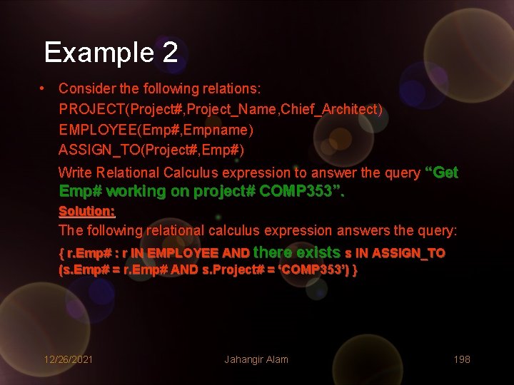
Example 2 • Consider the following relations: PROJECT(Project#, Project_Name, Chief_Architect) EMPLOYEE(Emp#, Empname) ASSIGN_TO(Project#, Emp#) Write Relational Calculus expression to answer the query “Get Emp# working on project# COMP 353”. Solution: The following relational calculus expression answers the query: { r. Emp# : r IN EMPLOYEE AND there exists s IN ASSIGN_TO (s. Emp# = r. Emp# AND s. Project# = ‘COMP 353’) } 12/26/2021 Jahangir Alam 198

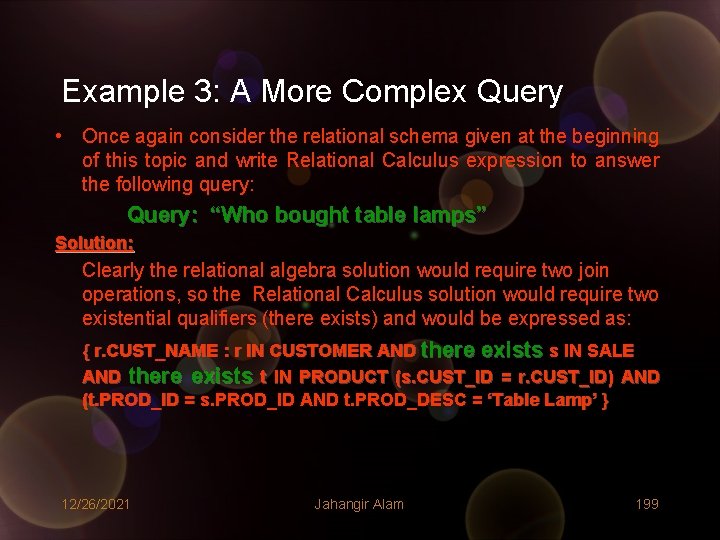
Example 3: A More Complex Query • Once again consider the relational schema given at the beginning of this topic and write Relational Calculus expression to answer the following query: Query: “Who bought table lamps” Solution: Clearly the relational algebra solution would require two join operations, so the Relational Calculus solution would require two existential qualifiers (there exists) and would be expressed as: { r. CUST_NAME : r IN CUSTOMER AND there exists s IN SALE AND there exists t IN PRODUCT (s. CUST_ID = r. CUST_ID) AND (t. PROD_ID = s. PROD_ID AND t. PROD_DESC = ‘Table Lamp’ } 12/26/2021 Jahangir Alam 199

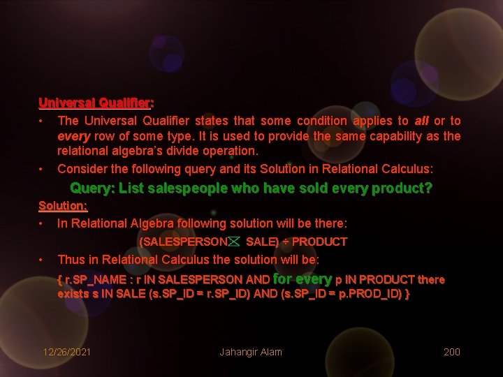
Universal Qualifier: • The Universal Qualifier states that some condition applies to all or to every row of some type. It is used to provide the same capability as the relational algebra’s divide operation. • Consider the following query and its Solution in Relational Calculus: Query: List salespeople who have sold every product? Solution: • In Relational Algebra following solution will be there: (SALESPERSON • SALE) ÷ PRODUCT Thus in Relational Calculus the solution will be: { r. SP_NAME : r IN SALESPERSON AND for every p IN PRODUCT there exists s IN SALE (s. SP_ID = r. SP_ID) AND (s. SP_ID = p. PROD_ID) } 12/26/2021 Jahangir Alam 200