DATA MINING SUPERVISED LEARNING Regression Classification Decision Trees

Supervised learning • In supervised learning, except for the feature variables that describe the

Applications • Descriptive modeling: Explanatory tool to understand the data: • Regression: How does

Supervised Learning Overview Learning algorithm Training data Model Train Apply Predict Test data Evaluate

Outliers • Regression is sensitive to outliers: • The line will “tilt” to accommodate

Normalization • In the regression problem some times our features may have very different

Interpretation and significance • Predicting Crime rate

Classification • Similar to the regression problem we have features and a target variable

Example: Catching tax-evasion Tax-return data for year 2011 A new tax return for 2012

Classification • Classification is the task of learning a target function f that maps

Examples of Classification Tasks • Predicting tumor cells as benign or malignant • Classifying

General approach to classification • Obtain a training set consisting of records with known

Evaluation of classification models • Counts of test records that are correctly (or incorrectly)

Classification Techniques • Decision Tree based Methods • Rule-based Methods • Memory based reasoning

Decision Trees • Decision tree • A flow-chart-like tree structure • Internal node denotes

Example of a Decision Tree o g te ca l l ir ca o

Another Example of Decision Tree l l a ric o ca g te o

Decision Tree Classification Task Decision Tree

Apply Model to Test Data Start from the root of tree. Refund Yes No

Apply Model to Test Data Refund Yes No NO Mar. St Single, Divorced Tax.

Tree Induction • Goal: Find the tree that has low classification error in the

General Structure of Hunt’s Algorithm • ?

Hunt’s Algorithm Don’t Cheat Refund Yes Don’t Cheat No Don’t Cheat Refund Yes No

Constructing decision-trees (pseudocode) Gen. Dec. Tree(Sample S, Features F) 1. If stopping_condition(S, F) =

Tree Induction • Issues • How to Classify a leaf node • Assign the

How to Specify Test Condition? • Depends on attribute types • Nominal • Ordinal

Splitting Based on Nominal Attributes • Multi-way split: Use as many partitions as distinct

Splitting Based on Ordinal Attributes • Multi-way split: Use as many partitions as distinct

Splitting Based on Continuous Attributes • Different ways of handling • Discretization to form

Splitting Based on Continuous Attributes

How to determine the Best Split Before Splitting: 10 records of class 0, 10

How to determine the Best Split • Greedy approach: • Creation of nodes with

Example: C 4. 5 • Simple depth-first construction. • Uses Information Gain • Sorts

Expressiveness • A classifier defines a function that discriminates between two (or more) classes.

Decision Boundary for Decision Trees • Consider a decision tree on real data where

Limitations of single attribute-based decision boundaries Both positive (+) and negative (o) classes generated

Oblique Decision Trees x+y<1 Class = + • Test condition may involve multiple attributes

Expressiveness • Decision tree provides expressive representation for learning discrete-valued function • But they

Instance-Based Classifiers • Store the training records • Use training records to predict the

Instance Based Classifiers • Examples: • Rote-learner • Memorizes entire training data and performs

Nearest Neighbor Classifiers • Basic idea: • “If it walks like a duck, quacks

Nearest-Neighbor Classifiers l Requires three things – The set of stored records – Distance

Definition of Nearest Neighbor K-nearest neighbors of a record x are data points that

1 nearest-neighbor Voronoi Diagram defines the classification boundary The area takes the class of

Nearest Neighbor Classification… • Choosing the value of k: • If k is too

Nearest Neighbor Classification… • Problem with Euclidean measure: • High dimensional data • curse

Nearest neighbor Classification… • k-NN classifiers are lazy learners • It does not build

Linear classifiers • SVMs are part of a family of classifiers that assumes that

Support Vector Machines • Find a linear hyperplane (decision boundary) that will separate the

Support Vector Machines • One Possible Solution

Support Vector Machines • Another possible solution

Support Vector Machines • Other possible solutions

Support Vector Machines • Which one is better? B 1 or B 2? •

Support Vector Machines • Find hyperplane maximizes the margin : B 1 is better

Support Vector Machines • What if the problem is not linearly separable?

Nonlinear Support Vector Machines • What if decision boundary is not linear?

Nonlinear Support Vector Machines • Trick: Transform data into higher dimensional space

Classification via regression • Instead of predicting the class of a record we want

Linear regression • A simple approach: use linear regression to learn a linear function

Logistic Regression Class Probabilities Linear regression on the log-odds ratio

Class probabilities for multiple dimensions • Assume a linear classification boundary

Logistic regression in 2 -d Coefficients

Logistic Regression • Produces a probability estimate for the class membership which is often

Bayesian Classifiers • How to classify the new record X = (‘Yes’, ‘Single’, 80

Bayesian Classifiers • In order for probabilities to be well defined: • Consider each

Example • Record X = (Refund = Yes, Status = Single, Income =80 K)

How to Estimate Probabilities from Data? •

Example of Naïve Bayes Classifier • Creating a Naïve Bayes Classifier, essentially means to

Example of Naïve Bayes Classifier Given a Test Record: X = (Refund = Yes,

Example of Naïve Bayes Classifier With Laplace Smoothing Given a Test Record: X =

Naïve Bayes for Text Classification • Fraction of documents in c Laplace Smoothing Total

Example News titles for Politics and Sports Politics documents “Obama meets Merkel” “Obama elected

Naïve Bayes (Summary) • Robust to isolated noise points • Handle missing values by

Generative vs Discriminative models • Naïve Bayes is a type of a generative model

Generative vs Discriminative models • Logistic Regression and SVM are discriminative models • The

Slides: 127

Download presentation

DATA MINING SUPERVISED LEARNING Regression Classification Decision Trees Classifier Expressiveness Nearest Neighbor Classifier Support Vector Machines (SVM) Logistic Regression Naïve Bayes

Supervised learning • In supervised learning, except for the feature variables that describe the data, we also have a target variable • The goal is to learn a function (model) that can estimate/predict the value of the target variable given the features • We learn the function using a labeled training set. • Regression: The target variable (but also the features) is numerical and continuous • The price of a stock, the GDP of a country, the grade in a class, the height of a child, the life expectancy etc • Classification: The target variable is discrete • Does a taxpayer cheat or not? Will the stock go up or down? Will the student pass or fail? Is a transaction fraudulent or not? What is the topic of an article?

Applications • Descriptive modeling: Explanatory tool to understand the data: • Regression: How does the change in the value of different factors affect our target variable? • What factors contribute to the price of a stock? • What factors contribute to the GDP of a country? • Classification: Understand what attributes distinguish between objects of different classes • Why people cheat on their taxes? • What words make an post offensive? • Predictive modeling: Predict a class of a previously unseen record • Regression: What will the life-expectancy of a patient be? • Classification: Is this a cheater or not? Will the stock go up or not. Is this an offensive post? • Predictive modeling is in the heart of the data science revolution.

Supervised Learning Overview Learning algorithm Training data Model Train Apply Predict Test data Evaluate

LINEAR REGRESSION

Regression •

Linear regression •

One-dimensional linear regression

Multiple linear regression •

Outliers • Regression is sensitive to outliers: • The line will “tilt” to accommodate very extreme values • Solution: remove the outliers • But make sure that they do not capture useful information

Normalization • In the regression problem some times our features may have very different scales: • For example: predict the GDP of a country using as features the percentage of home owners and the income • The weights in this case will not be interpretable • Solution: Normalize the features by replacing the values with the z -scores • Remove the mean and divide by the standard deviation

More complex models •

Interpretation and significance • Predicting Crime rate

CLASSIFICATION

Classification • Similar to the regression problem we have features and a target variable that we want to model/predict • The target variable is now discrete. It is often called the class label • In the simplest case, it is a binary variable. • In classification the features may also be categorical.

Example: Catching tax-evasion Tax-return data for year 2011 A new tax return for 2012 Is this a cheating tax return? An instance of the classification problem: learn a method for discriminating between records of different classes (cheaters vs non-cheaters)

Classification • Classification is the task of learning a target function f that maps attribute set x to one of the predefined class labels y • The function may be defined as an algorithm (e. g. , if Single and Income < 125 K then No) l o ca g te l a ric o g te ca s a ric in u uo c t on s s cla One of the attributes is the class attribute In this case: Cheat Two class labels (or classes): Yes (1), No (0)

Examples of Classification Tasks • Predicting tumor cells as benign or malignant • Classifying credit card transactions as legitimate or fraudulent • Categorizing news stories as finance, weather, entertainment, sports • Identifying spam email, spam web pages, adult content • Understanding if a web query has commercial intent or not Classification is everywhere in data science Big data has the answers to all questions.

General approach to classification • Obtain a training set consisting of records with known class labels • Training set is used to build a classification model • A labeled test set of previously unseen data records is used to evaluate the quality of the model. • The classification model is applied to new records with unknown class labels • Important intermediate step: Decide on what features to use

Illustrating Classification Task

Evaluation of classification models • Counts of test records that are correctly (or incorrectly) predicted by Actual Class the classification model • Confusion matrix Predicted Class = 1 Class = 0 Class = 1 f 10 Class = 0 f 01 f 00

Classification Techniques • Decision Tree based Methods • Rule-based Methods • Memory based reasoning • Neural Networks • Naïve Bayes and Bayesian Belief Networks • Support Vector Machines • Logistic Regression

DECISION TREES

Decision Trees • Decision tree • A flow-chart-like tree structure • Internal node denotes a test on an attribute • Branch represents an outcome of the test • Leaf nodes represent class labels or class distribution

Example of a Decision Tree o g te ca l l ir ca o g te ca s a ric in u uo c t on ss cla Splitting Attributes Refund Yes No NO Mar. St Test outcome Married Single, Divorced Tax. Inc < 80 K NO NO > 80 K YES Class labels Training Data Model: Decision Tree

Another Example of Decision Tree l l a ric o ca g te o g te ca s a ric in u uo c t on ss cla Married Mar. St NO Single, Divorced Refund No Yes NO Tax. Inc < 80 K NO > 80 K YES There could be more than one tree that fits the same data!

Decision Tree Classification Task Decision Tree

Apply Model to Test Data Start from the root of tree. Refund Yes No NO Mar. St Single, Divorced Tax. Inc < 80 K NO Married NO > 80 K YES

Apply Model to Test Data Refund Yes No NO Mar. St Single, Divorced Tax. Inc < 80 K NO Married NO > 80 K YES

Apply Model to Test Data Refund Yes No NO Mar. St Single, Divorced Tax. Inc < 80 K NO Married NO > 80 K YES Assign Cheat to “No”

Decision Tree Classification Task Decision Tree

Tree Induction • Goal: Find the tree that has low classification error in the training data (training error) • Finding the best decision tree (lowest training error) is NP-hard • Greedy strategy. • Split the records based on an attribute test that optimizes certain criterion. • Many Algorithms: • Hunt’s Algorithm (one of the earliest) • CART • ID 3, C 4. 5 • SLIQ, SPRINT

General Structure of Hunt’s Algorithm • ?

Hunt’s Algorithm Don’t Cheat Refund Yes Don’t Cheat No Don’t Cheat Refund Yes No Don’t Marital Cheat Status Single, Married Divorced Don’t Cheat Yes No Don’t Marital Cheat Status Single, Married Divorced Don’t Taxable Cheat Income < 80 K Don’t Cheat >= 80 K Cheat

Constructing decision-trees (pseudocode) Gen. Dec. Tree(Sample S, Features F) 1. If stopping_condition(S, F) = true then a. b. c. 2. 3. 4. 5. root = create. Node() root. test_condition = find. Best. Split(S, F) V = {v| v a possible outcome of root. test_condition} for each value vєV: a. b. c. 6. leaf = create. Node() leaf. label= Classify(S) return leaf Sv: = {s | root. test_condition(s) = v and s є S}; child = Gen. Dec. Tree(Sv , F) ; Add child as a descent of root and label the edge (root child) as v return root

Tree Induction • Issues • How to Classify a leaf node • Assign the majority class • If leaf is empty, assign the default class – the class that has the highest popularity (overall or in the parent node). • Determine how to split the records • How to specify the attribute test condition? • How to determine the best split? • Determine when to stop splitting

How to Specify Test Condition? • Depends on attribute types • Nominal • Ordinal • Continuous • Depends on number of ways to split • 2 -way split • Multi-way split

Splitting Based on Nominal Attributes • Multi-way split: Use as many partitions as distinct values. Car. Type Family Luxury Sports • Binary split: Divides values into two subsets. Need to find optimal partitioning. {Sports, Luxury} Car. Type {Family} OR {Family, Luxury} Car. Type {Sports}

Splitting Based on Ordinal Attributes • Multi-way split: Use as many partitions as distinct values. Size Small Medium Large • Binary split: Divides values into two subsets – respects the order. Need to find optimal partitioning. {Small, Medium} Size {Large} OR • What about this split? {Small, Large} {Medium, Large} Size {Medium} {Small}

Splitting Based on Continuous Attributes • Different ways of handling • Discretization to form an ordinal categorical attribute • Static – discretize once at the beginning • Dynamic – ranges can be found by equal interval bucketing, equal frequency bucketing (percentiles), or clustering. • Binary Decision: (A < v) or (A v) • consider all possible splits and finds the best cut • can be more computationally intensive

Splitting Based on Continuous Attributes

How to determine the Best Split Before Splitting: 10 records of class 0, 10 records of class 1 Which test condition is the best?

How to determine the Best Split • Greedy approach: • Creation of nodes with homogeneous class distribution is preferred • Need a measure of node impurity: • Ideas? Non-homogeneous, High degree of impurity Low degree of impurity

Measuring Node Impurity •

Example: C 4. 5 • Simple depth-first construction. • Uses Information Gain • Sorts Continuous Attributes at each node. • Needs entire data to fit in memory. • Unsuitable for Large Datasets. • Needs out-of-core sorting. • You can download the software from: http: //www. cse. unsw. edu. au/~quinlan/c 4. 5 r 8. tar. gz

EXPRESSIVENESS

Expressiveness • A classifier defines a function that discriminates between two (or more) classes. • The expressiveness of a classifier is the class of functions that it can model, and the kind of data that it can separate • When we have discrete (or binary) values, we are interested in the class of boolean functions that can be modeled • When the data-points are real vectors we talk about the decision boundary that the classifier can model • The decision boundary is the (multi-dimensional) surface defined by the function of the classifier that separates the YES and NO decisions

Decision Boundary for Decision Trees • Consider a decision tree on real data where the test conditions involve a single attribute at a time, and a Yes/No question • Each test defines a line parallel to an axis (the one corresponding to the test attribute) • The decision boundary is a collection of lines parallel to the axes

Limitations of single attribute-based decision boundaries Both positive (+) and negative (o) classes generated from skewed Gaussians with centers at (8, 8) and (12, 12) respectively. The resulting boundary is very complex.

Oblique Decision Trees x+y<1 Class = + • Test condition may involve multiple attributes • More expressive representation • Finding optimal test condition is computationally expensive Class =

Expressiveness • Decision tree provides expressive representation for learning discrete-valued function • But they do not generalize well to certain types of Boolean functions • Example: parity function: • Class = 1 if there is an even number of Boolean attributes with truth value = True • Class = 0 if there is an odd number of Boolean attributes with truth value = True • For accurate modeling, must have a complete tree • Less expressive for modeling continuous variables • Particularly when test condition involves only a single attribute at-a-time

NEAREST NEIGHBOR CLASSIFICATION

Instance-Based Classifiers • Store the training records • Use training records to predict the class label of unseen cases

Instance Based Classifiers • Examples: • Rote-learner • Memorizes entire training data and performs classification only if attributes of record match one of the training examples exactly • Nearest neighbor classifier • Uses k “closest” points (nearest neighbors) for performing classification

Nearest Neighbor Classifiers • Basic idea: • “If it walks like a duck, quacks like a duck, then it’s probably a duck” Compute Distance Training Records Choose k of the “nearest” records Test Record

Nearest-Neighbor Classifiers l Requires three things – The set of stored records – Distance Metric to compute distance between records – The value of k, the number of nearest neighbors to retrieve l To classify an unknown record: 1. Compute distance to other training records 2. Identify k nearest neighbors 3. Use class labels of nearest neighbors to determine the class label of unknown record (e. g. , by taking majority vote)

Nearest Neighbor Classification •

Definition of Nearest Neighbor K-nearest neighbors of a record x are data points that have the k smallest distance to x

1 nearest-neighbor Voronoi Diagram defines the classification boundary The area takes the class of the green point

Nearest Neighbor Classification… • Choosing the value of k: • If k is too small, sensitive to noise points • If k is too large, neighborhood may include points from other classes The value of k determines the complexity of the model Lower k produces more complex models

Example

Nearest Neighbor Classification… • Problem with Euclidean measure: • High dimensional data • curse of dimensionality • Can produce counter-intuitive results 1111110 u vs 1000000 0111111 0000001 d = 1. 4142 Solution: Normalize the vectors to unit length

Nearest neighbor Classification… • k-NN classifiers are lazy learners • It does not build models explicitly • Unlike eager learners such as decision trees • Classifying unknown records is relatively expensive • Naïve algorithm: O(n) • Need for structures to retrieve nearest neighbors fast. • The Nearest Neighbor Search problem. • Also, Approximate Nearest Neighbor Search • Issues with distance in very high-dimensional spaces

SUPPORT VECTOR MACHINES

Linear classifiers • SVMs are part of a family of classifiers that assumes that the classes are linearly separable • That is, there is a hyperplane that separates (approximately, or exactly) the instances of the two classes. • The goal is to find this hyperplane

Support Vector Machines • Find a linear hyperplane (decision boundary) that will separate the data

Support Vector Machines • One Possible Solution

Support Vector Machines • Another possible solution

Support Vector Machines • Other possible solutions

Support Vector Machines • Which one is better? B 1 or B 2? • How do you define better?

Support Vector Machines • Find hyperplane maximizes the margin : B 1 is better than B 2

Support Vector Machines

Support Vector Machines •

Support Vector Machines • What if the problem is not linearly separable?

Support Vector Machines •

Nonlinear Support Vector Machines • What if decision boundary is not linear?

Nonlinear Support Vector Machines • Trick: Transform data into higher dimensional space

Learning Nonlinear SVM •

Learning Non. Linear SVM •

Learning Nonlinear SVM •

Example of Nonlinear SVM

Learning Nonlinear SVM •

LOGISTIC REGRESSION

Classification via regression • Instead of predicting the class of a record we want to predict the probability of the class given the record • Transform the classification problem into a regression problem. • But how do you define the probability that you want to predict?

Linear regression • A simple approach: use linear regression to learn a linear function that predicts 0/1 values • Not good: It may produce negative probabilities, or probabilities that are greater than 1. • Also the probabilities it produces are not what we want. We want probability close to zero for small values, and close to 1 for large, and a transition from 0 to 1 around the value 20

The logistic function

Logistic Regression Class Probabilities Linear regression on the log-odds ratio

Logistic Regression in one dimension

Class probabilities for multiple dimensions • Assume a linear classification boundary

Logistic Regression Class probabilities Linear regression on the log-odds ratio

Logistic regression in 2 -d Coefficients

Estimating the coefficients •

Logistic Regression • Produces a probability estimate for the class membership which is often very useful. • The weights can be useful for understanding the feature importance. • Works for relatively large datasets • Fast to apply.

NAÏVE BAYES CLASSIFIER

Bayes Classifier •

Bayesian Classifiers • How to classify the new record X = (‘Yes’, ‘Single’, 80 K) Find the class with the highest probability given the vector values. Maximum Aposteriori Probability estimate: • Find the value c for class C that maximizes P(C=c| X) • How do we estimate P(C|X) for the different values of C? • We want to estimate • P(C=Yes| X) • P(C=No| X)

Bayesian Classifiers • In order for probabilities to be well defined: • Consider each attribute and the class label as random variables • Probabilities are determined from the data

Bayesian Classifiers •

Naïve Bayes Classifier •

How to Estimate Probabilities from Data? •

Example of Naïve Bayes Classifier • Creating a Naïve Bayes Classifier, essentially means to compute counts: Total number of records: N = 10 Class No: Number of records: 7 Attribute Refund: Yes: 3 No: 4 Attribute Marital Status: Single: 2 Divorced: 1 Married: 4 Attribute Income: mean: 110 variance: 2975 Class Yes: Number of records: 3 Attribute Refund: Yes: 0 No: 3 Attribute Marital Status: Single: 2 Divorced: 1 Married: 0 Attribute Income: mean: 90 variance: 25

Naïve Bayes Classifier •

Example of Naïve Bayes Classifier • Creating a Naïve Bayes Classifier, essentially means to compute counts: With Laplace Smoothing Total number of records: N = 10 Class No: Number of records: 7 Attribute Refund: Yes: 3 No: 4 Attribute Marital Status: Single: 2 Divorced: 1 Married: 4 Attribute Income: mean: 110 variance: 2975 Class Yes: Number of records: 3 Attribute Refund: Yes: 0 No: 3 Attribute Marital Status: Single: 2 Divorced: 1 Married: 0 Attribute Income: mean: 90 variance: 25

Implementation details •

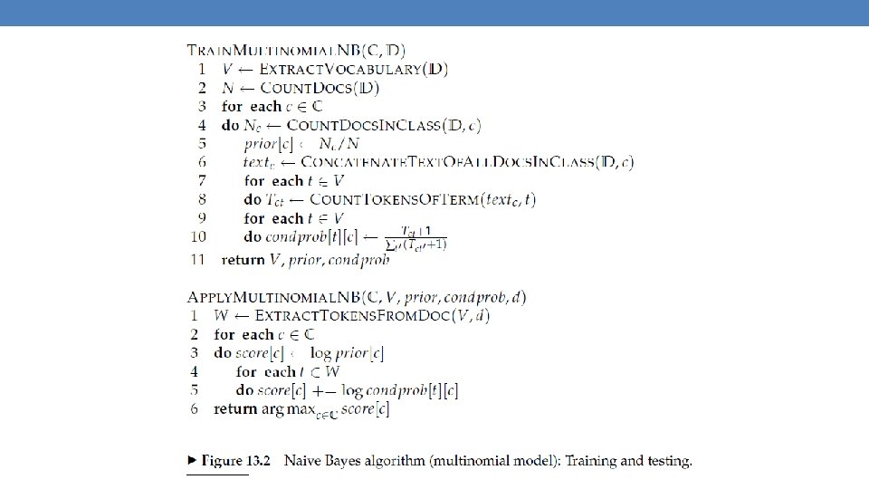
Naïve Bayes for Text Classification • Fraction of documents in c Laplace Smoothing Total number of terms in all documents in c Number of unique words (vocabulary size)

Multinomial document model • w

Example News titles for Politics and Sports Politics documents “Obama meets Merkel” “Obama elected again” “Merkel visits Greece again” P(p) = 0. 5 obama: 2, meets: 1, merkel: 2, Vocabulary elected: 1, again: 2, visits: 1, greece: 1 size: 14 terms Total terms: 10 New title: Sports “OSFP European basketball champion” “Miami NBA basketball champion” “Greece basketball coach? ” P(s) = 0. 5 OSFP: 1, european: 1, basketball: 3, champion: 2, miami: 1, nba: 1, greece: 1, coach: 1 Total terms: 11 X = “Obama likes basketball” P(Politics|X) ~ P(p)*P(obama|p)*P(likes|p)*P(basketball|p) = 0. 5 * 3/(10+14) *1/(10+14) * 1/(10+14) = 0. 000108 P(Sports|X) ~ P(s)*P(obama|s)*P(likes|s)*P(basketball|s) = 0. 5 * 1/(11+14) * 4/(11+14) = 0. 000128

Naïve Bayes (Summary) • Robust to isolated noise points • Handle missing values by ignoring the instance during probability estimate calculations • Robust to irrelevant attributes • Independence assumption may not hold for some attributes • Use other techniques such as Bayesian Belief Networks (BBN) • Naïve Bayes can produce a probability estimate, but it is usually a very biased one • Logistic Regression is better for obtaining probabilities.

Generative vs Discriminative models • Naïve Bayes is a type of a generative model • Generative process: • First pick the category of the record • Then given the category, generate the attribute values from the distribution of the category C • Conditional independence given C • We use the training data to learn the distributions most likely to have generated the data

Generative vs Discriminative models • Logistic Regression and SVM are discriminative models • The goal is to find the boundary that discriminates between the two classes from the training data • In order to classify the language of a document, you can • Either learn the two languages and find which is more likely to have generated the words you see • Or learn what differentiates the two languages.