Data Mining Practical Machine Learning Tools and Techniques

Data Mining Practical Machine Learning Tools and Techniques Slides for Chapter 2, Input: concepts, instances, attributes of Data Mining by I. H. Witten, E. Frank, M. A. Hall and C. J. Pal

Input: concepts, instances, attributes • Components of the input for learning • What’s a concept? • Classification, association, clustering, numeric prediction • What’s in an example? • Relations, flat files, recursion • What’s in an attribute? • Nominal, ordinal, interval, ratio • Preparing the input • ARFF, sparse data, attributes, missing and inaccurate values, unbalanced data, getting to know your data 2

Components of the input • Concepts: kinds of things that can be learned • Aim: intelligible and operational concept description • Instances: the individual, independent examples of a concept to be learned • More complicated forms of input with dependencies between examples are possible • Attributes: measuring aspects of an instance • We will focus on nominal and numeric ones 3

What’s a concept? • Concept: thing to be learned • Concept description: output of learning scheme • Styles of learning: • Classification learning: predicting a discrete class • Association learning: detecting associations between features • Clustering: grouping similar instances into clusters • Numeric prediction: predicting a numeric quantity 4

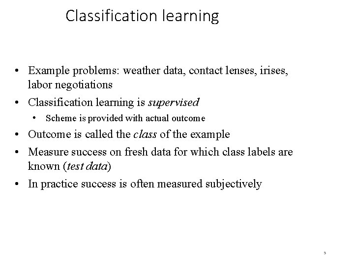
Classification learning • Example problems: weather data, contact lenses, irises, labor negotiations • Classification learning is supervised • Scheme is provided with actual outcome • Outcome is called the class of the example • Measure success on fresh data for which class labels are known (test data) • In practice success is often measured subjectively 5

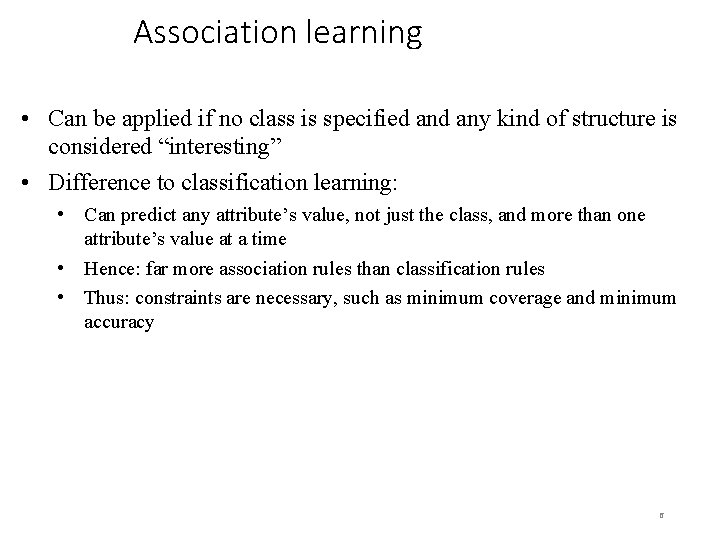
Association learning • Can be applied if no class is specified any kind of structure is considered “interesting” • Difference to classification learning: • Can predict any attribute’s value, not just the class, and more than one attribute’s value at a time • Hence: far more association rules than classification rules • Thus: constraints are necessary, such as minimum coverage and minimum accuracy 6

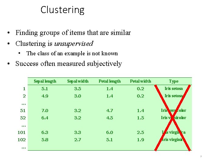
Clustering • Finding groups of items that are similar • Clustering is unsupervised • The class of an example is not known • Success often measured subjectively Sepal length Sepal width Petal length Petal width Type 1 5. 1 3. 5 1. 4 0. 2 Iris setosa 2 4. 9 3. 0 1. 4 0. 2 Iris setosa 51 7. 0 3. 2 4. 7 1. 4 Iris versicolor 52 6. 4 3. 2 4. 5 1. 5 Iris versicolor 101 6. 3 3. 3 6. 0 2. 5 Iris virginica 102 5. 8 2. 7 5. 1 1. 9 Iris virginica … … … 7

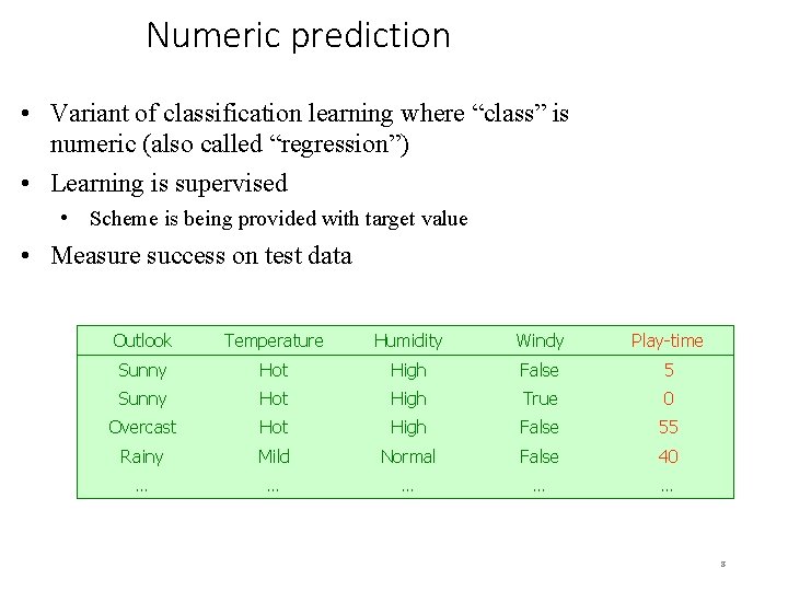
Numeric prediction • Variant of classification learning where “class” is numeric (also called “regression”) • Learning is supervised • Scheme is being provided with target value • Measure success on test data Outlook Temperature Humidity Windy Play-time Sunny Hot High False 5 Sunny Hot High True 0 Overcast Hot High False 55 Rainy Mild Normal False 40 … … … 8

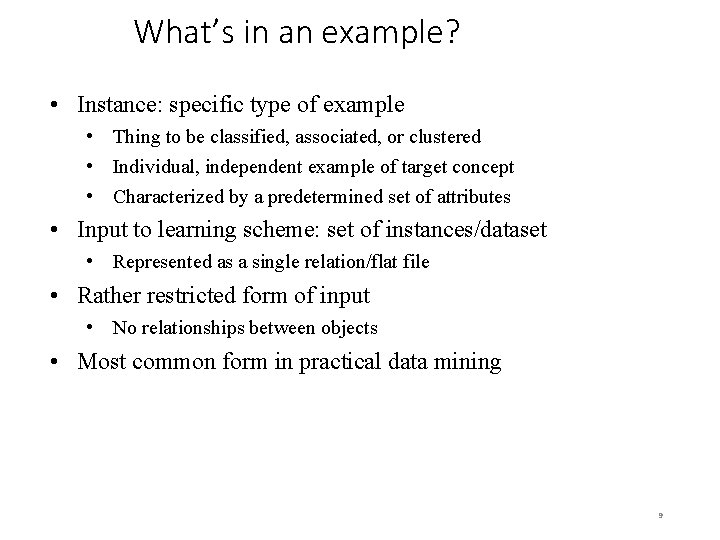
What’s in an example? • Instance: specific type of example • Thing to be classified, associated, or clustered • Individual, independent example of target concept • Characterized by a predetermined set of attributes • Input to learning scheme: set of instances/dataset • Represented as a single relation/flat file • Rather restricted form of input • No relationships between objects • Most common form in practical data mining 9

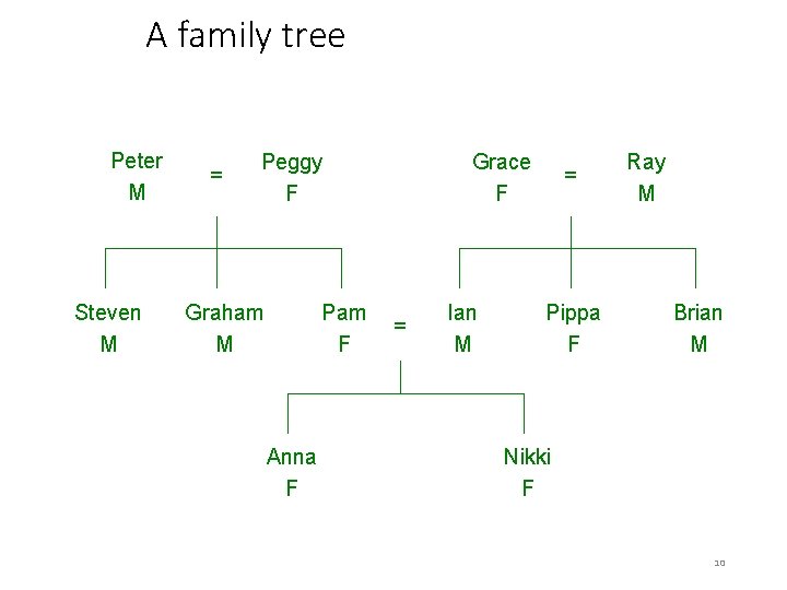
A family tree Peter M Steven M = Peggy F Graham M Pam F Anna F Grace F = Ian M = Pippa F Ray M Brian M Nikki F 10

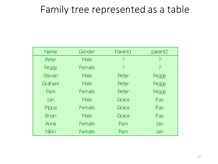
Family tree represented as a table Name Gender Parent 1 parent 2 Peter Male ? ? Peggy Female ? ? Steven Male Peter Peggy Graham Male Peter Peggy Pam Female Peter Peggy Ian Male Grace Ray Pippa Female Grace Ray Brian Male Grace Ray Anna Female Pam Ian Nikki Female Pam Ian 11

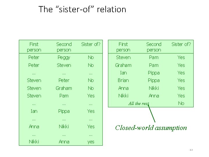
The “sister-of” relation First person Second person Sister of? Peter Peggy No Steven Pam Yes Peter Steven No Graham Pam Yes … … … Ian Pippa Yes Steven Peter No Brian Pippa Yes Steven Graham No Anna Nikki Yes Steven Pam Yes Nikki Anna Yes … … … Ian Pippa Yes … … … Anna Nikki Yes … … … Nikki Anna yes All the rest No Closed-world assumption 12

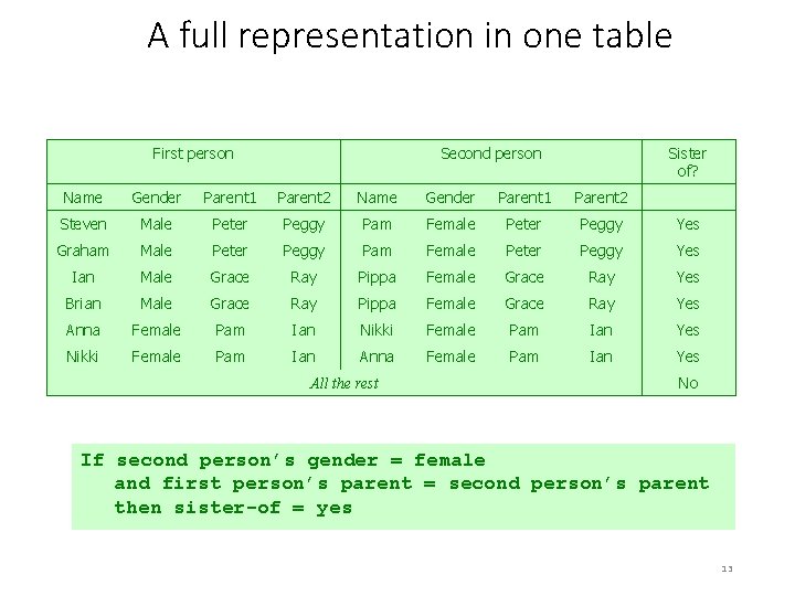
A full representation in one table First person Second person Sister of? Name Gender Parent 1 Parent 2 Steven Male Peter Peggy Pam Female Peter Peggy Yes Graham Male Peter Peggy Pam Female Peter Peggy Yes Ian Male Grace Ray Pippa Female Grace Ray Yes Brian Male Grace Ray Pippa Female Grace Ray Yes Anna Female Pam Ian Nikki Female Pam Ian Yes Nikki Female Pam Ian Anna Female Pam Ian Yes All the rest No If second person’s gender = female and first person’s parent = second person’s parent then sister-of = yes 13

Generating a flat file • Process of flattening called “denormalization” • Several relations are joined together to make one • Possible with any finite set of finite relations • Problematic: relationships without a pre-specified number of objects • Example: concept of nuclear-family • Note that denormalization may produce spurious regularities that reflect the structure of the database • Example: “supplier” predicts “supplier address” 14

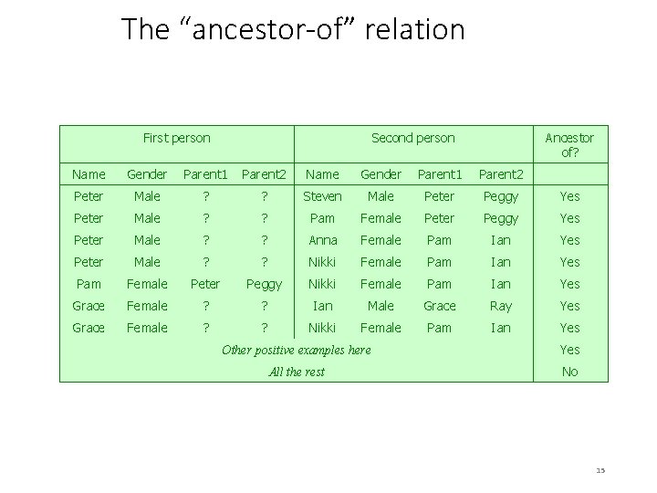
The “ancestor-of” relation First person Second person Ancestor of? Name Gender Parent 1 Parent 2 Peter Male ? ? Steven Male Peter Peggy Yes Peter Male ? ? Pam Female Peter Peggy Yes Peter Male ? ? Anna Female Pam Ian Yes Peter Male ? ? Nikki Female Pam Ian Yes Pam Female Peter Peggy Nikki Female Pam Ian Yes Grace Female ? ? Ian Male Grace Ray Yes Grace Female ? ? Nikki Female Pam Ian Yes Other positive examples here Yes All the rest No 15

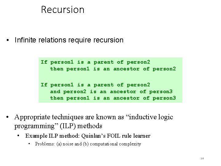
Recursion • Infinite relations require recursion If person 1 is a parent of person 2 then person 1 is an ancestor of person 2 If person 1 is a parent of person 2 and person 2 is an ancestor of person 3 then person 1 is an ancestor of person 3 • Appropriate techniques are known as “inductive logic programming” (ILP) methods • Example ILP method: Quinlan’s FOIL rule learner • Problems: (a) noise and (b) computational complexity 16

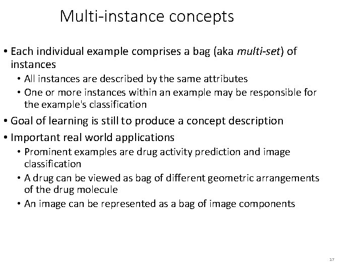
Multi-instance concepts • Each individual example comprises a bag (aka multi-set) of instances • All instances are described by the same attributes • One or more instances within an example may be responsible for the example's classification • Goal of learning is still to produce a concept description • Important real world applications • Prominent examples are drug activity prediction and image classification • A drug can be viewed as bag of different geometric arrangements of the drug molecule • An image can be represented as a bag of image components 17

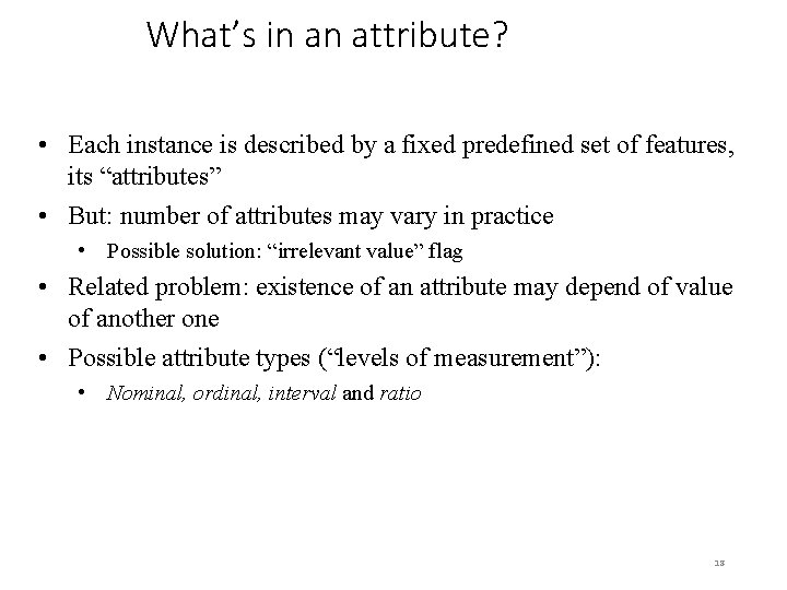
What’s in an attribute? • Each instance is described by a fixed predefined set of features, its “attributes” • But: number of attributes may vary in practice • Possible solution: “irrelevant value” flag • Related problem: existence of an attribute may depend of value of another one • Possible attribute types (“levels of measurement”): • Nominal, ordinal, interval and ratio 18

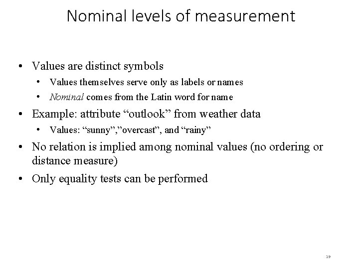
Nominal levels of measurement • Values are distinct symbols • Values themselves serve only as labels or names • Nominal comes from the Latin word for name • Example: attribute “outlook” from weather data • Values: “sunny”, ”overcast”, and “rainy” • No relation is implied among nominal values (no ordering or distance measure) • Only equality tests can be performed 19

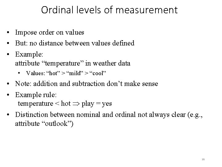
Ordinal levels of measurement • Impose order on values • But: no distance between values defined • Example: attribute “temperature” in weather data • Values: “hot” > “mild” > “cool” • Note: addition and subtraction don’t make sense • Example rule: temperature < hot play = yes • Distinction between nominal and ordinal not always clear (e. g. , attribute “outlook”) 20

Interval quantities • Interval quantities are not only ordered but measured in fixed and equal units • Example 1: attribute “temperature” expressed in degrees Fahrenheit • Example 2: attribute “year” • Difference of two values makes sense • Sum or product doesn’t make sense • Zero point is not defined! 21

Ratio quantities • Ratio quantities are ones for which the measurement scheme defines a zero point • Example: attribute “distance” • Distance between an object and itself is zero • Ratio quantities are treated as real numbers • All mathematical operations are allowed • But: is there an “inherently” defined zero point? • Answer depends on scientific knowledge (e. g. , Fahrenheit knew no lower limit to temperature) 22

Attribute types used in practice • Many data mining schemes accommodate just two levels of measurement: nominal and ordinal • Others deal exclusively with ratio quantities • Nominal attributes are also called “categorical”, ”enumerated”, or “discrete” • But: “enumerated” and “discrete” imply order • Special case: dichotomy (“boolean” attribute) • Ordinal attributes are sometimes coded as “numeric” or “continuous” • But: “continuous” implies mathematical continuity 23

Metadata • Information about the data that encodes background knowledge • In theory this information can be used to restrict the search space of the learning algorithm • Examples: • Dimensional considerations (i. e. , expressions must be dimensionally correct) • Circular orderings (e. g. , degrees in compass) • Partial orderings (e. g. , generalization/specialization relations) 24

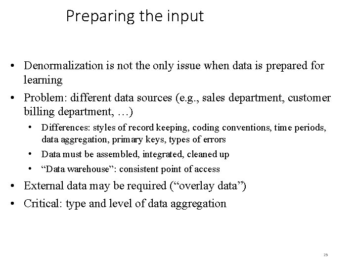
Preparing the input • Denormalization is not the only issue when data is prepared for learning • Problem: different data sources (e. g. , sales department, customer billing department, …) • Differences: styles of record keeping, coding conventions, time periods, data aggregation, primary keys, types of errors • Data must be assembled, integrated, cleaned up • “Data warehouse”: consistent point of access • External data may be required (“overlay data”) • Critical: type and level of data aggregation 25

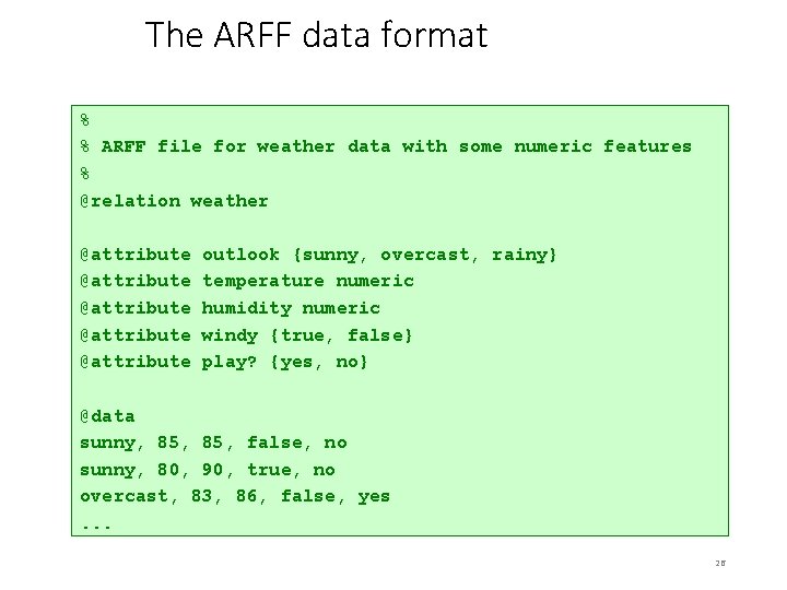
The ARFF data format % % ARFF file for weather data with some numeric features % @relation weather @attribute @attribute outlook {sunny, overcast, rainy} temperature numeric humidity numeric windy {true, false} play? {yes, no} @data sunny, 85, false, no sunny, 80, 90, true, no overcast, 83, 86, false, yes. . . 26

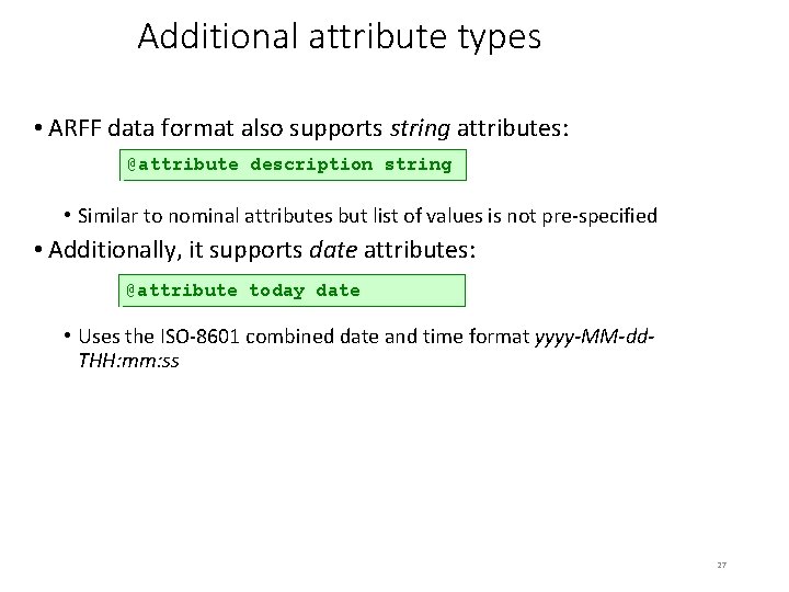
Additional attribute types • ARFF data format also supports string attributes: @attribute description string • Similar to nominal attributes but list of values is not pre-specified • Additionally, it supports date attributes: @attribute today date • Uses the ISO-8601 combined date and time format yyyy-MM-dd. THH: mm: ss 27

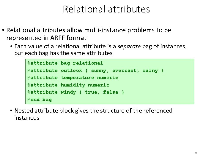
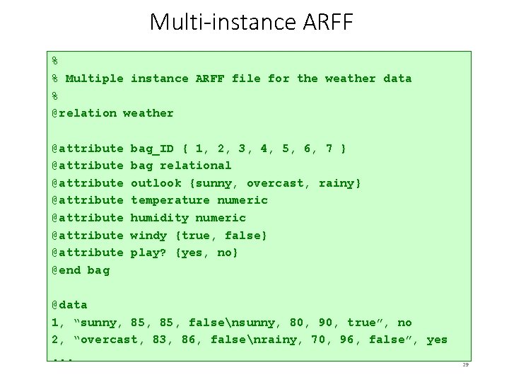
Relational attributes • Relational attributes allow multi-instance problems to be represented in ARFF format • Each value of a relational attribute is a separate bag of instances, but each bag has the same attributes @attribute @attribute @end bag relational outlook { sunny, overcast, rainy } temperature numeric humidity numeric windy { true, false } • Nested attribute block gives the structure of the referenced instances 28

Multi-instance ARFF % % Multiple instance ARFF file for the weather data % @relation weather @attribute @attribute @end bag_ID { 1, 2, 3, 4, 5, 6, 7 } bag relational outlook {sunny, overcast, rainy} temperature numeric humidity numeric windy {true, false} play? {yes, no} @data 1, “sunny, 85, falsensunny, 80, 90, true”, no 2, “overcast, 83, 86, falsenrainy, 70, 96, false”, yes. . . 29

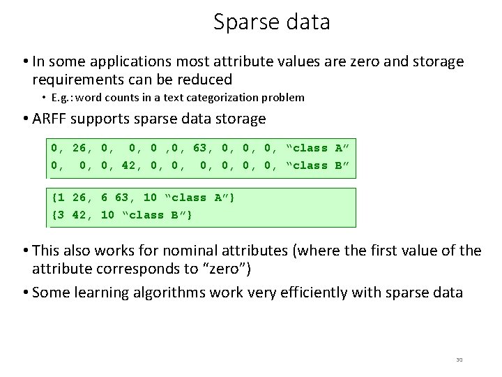
Sparse data • In some applications most attribute values are zero and storage requirements can be reduced • E. g. : word counts in a text categorization problem • ARFF supports sparse data storage 0, 26, 0, 0, 0 , 0, 63, 0, 0, 0, “class A” 0, 0, 0, 42, 0, 0, 0, “class B” {1 26, 6 63, 10 “class A”} {3 42, 10 “class B”} • This also works for nominal attributes (where the first value of the attribute corresponds to “zero”) • Some learning algorithms work very efficiently with sparse data 30

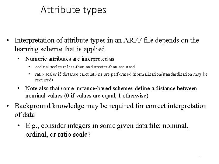
Attribute types • Interpretation of attribute types in an ARFF file depends on the learning scheme that is applied • Numeric attributes are interpreted as • • ordinal scales if less-than and greater-than are used ratio scales if distance calculations are performed (normalization/standardization may be required) • Note also that some instance-based schemes define a distance between nominal values (0 if values are equal, 1 otherwise) • Background knowledge may be required for correct interpretation of data • E. g. , consider integers in some given data file: nominal, ordinal, or ratio scale? 31

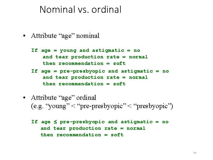
Nominal vs. ordinal • Attribute “age” nominal If age = young and astigmatic = no and tear production rate = normal then recommendation = soft If age = pre-presbyopic and astigmatic = no and tear production rate = normal then recommendation = soft • Attribute “age” ordinal (e. g. “young” < “pre-presbyopic” < “presbyopic”) If age pre-presbyopic and astigmatic = no and tear production rate = normal then recommendation = soft 32

Missing values • Missing values are frequently indicated by out-of-range entries for an attribute • There are different types of missing values: unknown, unrecorded, irrelevant • Reasons: • • malfunctioning equipment changes in experimental design collation of different datasets measurement not possible • Missing value may have significance in itself (e. g. , missing test in a medical examination) • Most schemes assume that is not the case and “missing” may need to be coded as an additional, separate attribute value 33

Inaccurate values • Reason: data has not been collected for mining it • Result: errors and omissions that affect the accuracy of data mining • These errors may not affect the original purpose of the data (e. g. , age of customer) • Typographical errors in nominal attributes values need to be checked for consistency • Typographical and measurement errors in numeric attributes outliers need to be identified • Errors may be deliberate (e. g. , wrong zip codes) • Other problems: duplicates, stale data 34

Unbalanced data • Unbalanced data is a well-known problem in classification problems • One class is often far more prevalent than the rest • Example: detecting a rare disease • Main problem: simply predicting the majority class yields high accuracy but is not useful • Predicting that no patient has the rare disease gives high classification accuracy • Unbalanced data requires techniques that can deal with unequal misclassification costs • Misclassifying an afflicted patient may be much more costly than misclassifying a healthy one 35

Getting to know your data • Simple visualization tools are very useful • Nominal attributes: histograms (Is the distribution consistent with background knowledge? ) • Numeric attributes: graphs (Any obvious outliers? ) • 2 -D and 3 -D plots show dependencies • May need to consult domain experts • Too much data to inspect manually? Take a sample! 36