Data Mining Practical Machine Learning Tools and Techniques

Data Mining Practical Machine Learning Tools and Techniques Slides for Chapter 7, Extending instance-based and linear models of Data Mining by I. H. Witten, E. Frank, M. A. Hall and C. J. Pal

Extending instance-based learning and linear models • Instance-based learning • Pruning and reducing the number of exemplars • Weighted attributes • Generalized exemplars and distance functions • Extending linear models • Support vector machines, kernel ridge regression, kernel perceptrons • Multilayer perceptrons and radial basis function networks • Gradient descent • Numeric prediction with local linear models • Model Trees • Learning rule sets with model trees • Locally weighted linear regression 2

Instance Based Learning 3

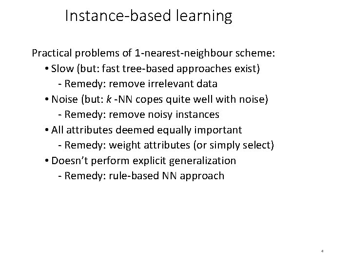
Instance-based learning Practical problems of 1 -nearest-neighbour scheme: • Slow (but: fast tree-based approaches exist) - Remedy: remove irrelevant data • Noise (but: k -NN copes quite well with noise) - Remedy: remove noisy instances • All attributes deemed equally important - Remedy: weight attributes (or simply select) • Doesn’t perform explicit generalization - Remedy: rule-based NN approach 4

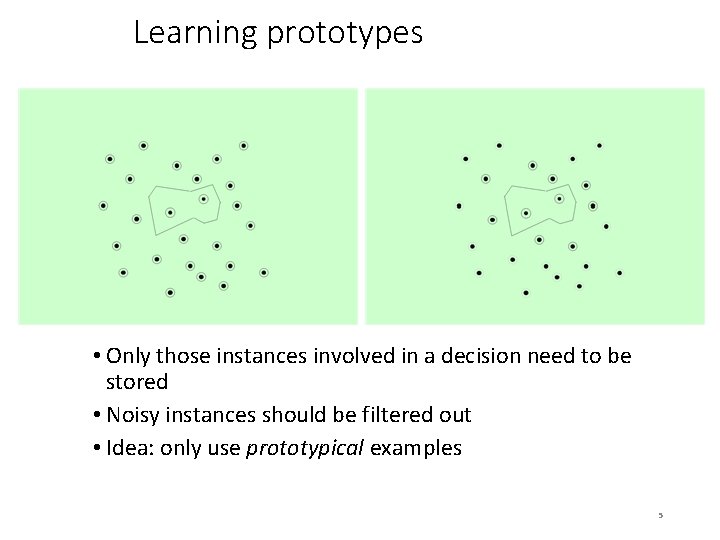
Learning prototypes • Only those instances involved in a decision need to be stored • Noisy instances should be filtered out • Idea: only use prototypical examples 5

Speed up classification, combat noise • David Aha’s IB 2: save memory, speed up classification • Work incrementally • Only incorporate misclassified instances • Problem: noisy data gets incorporated • David Aha’s IB 3: deal with noise • Discard instances that do not perform well • Compute confidence intervals for 1. Each instance’s success rate 2. Default accuracy of the instance’s class • Accept/reject instances according to performance 1. Accept if lower limit of 1 exceeds upper limit of 2 2. Reject if upper limit of 1 is below lower limit of 2 6

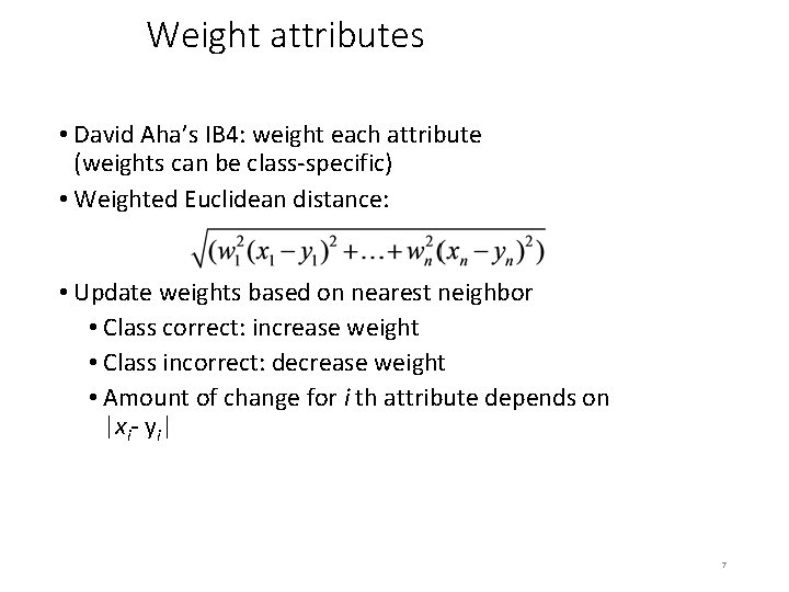
Weight attributes • David Aha’s IB 4: weight each attribute (weights can be class-specific) • Weighted Euclidean distance: • Update weights based on nearest neighbor • Class correct: increase weight • Class incorrect: decrease weight • Amount of change for i th attribute depends on |xi- yi| 7

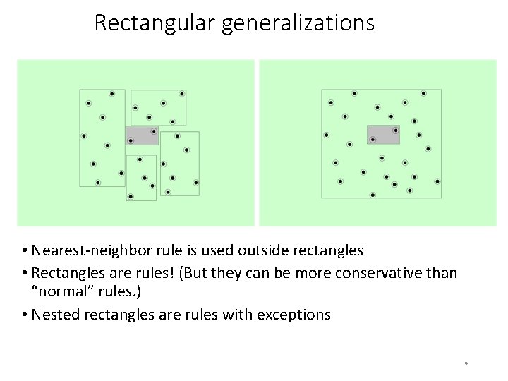
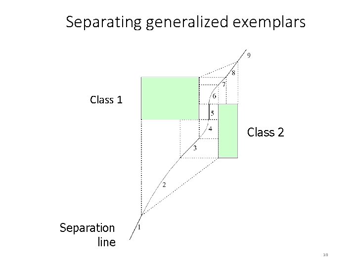
Generalized exemplars • Generalize instances into hyperrectangles • Online: incrementally modify rectangles • Offline version: seek small set of rectangles that cover the instances • Important design decisions: • Allow overlapping rectangles? • Requires conflict resolution • Allow nested rectangles? • Dealing with uncovered instances? 8

Rectangular generalizations • Nearest-neighbor rule is used outside rectangles • Rectangles are rules! (But they can be more conservative than “normal” rules. ) • Nested rectangles are rules with exceptions 9

Separating generalized exemplars Class 1 Class 2 Separation line 10

Generalized distance functions • Problem with Euclidean distance, etc. : only natural for purely numeric datasets • Transformation-based approach to designing distance functions can be applied more generally • Given: some transformation operations on attributes • K* similarity = probability of transforming instance A into B by chance • Average over all transformation paths • Weight paths according their probability (need way of measuring this) • Uniform way of dealing with different attribute types • Easily generalized to give distance between sets of instances 11

Discussion and Bibliographic Notes • Nearest-neighbor methods gained popularity in machine learning through the work of Aha (1992) • Salzberg (1991) suggested that generalization with nested exemplars can achieve high classification accuracy • Wettschereck and Dietterich (1994) argued that these results were fortuitous and did not hold in other domains • Martin (1995) explored the idea that overgeneralization that occurs when hyperrectangles nest or overlap is problematic • The generalized distance function based on transformations is described by Cleary and Trigg (1995) 12

Extending Linear Models 13

Support vector machines • Support vector machines are algorithms for learning linear classifiers • Resilient to overfitting because they learn a particular linear decision boundary: • The maximum margin hyperplane • Fast in the nonlinear case • Use a mathematical trick to avoid creating “pseudo-attributes” • The nonlinear space is created implicitly 14

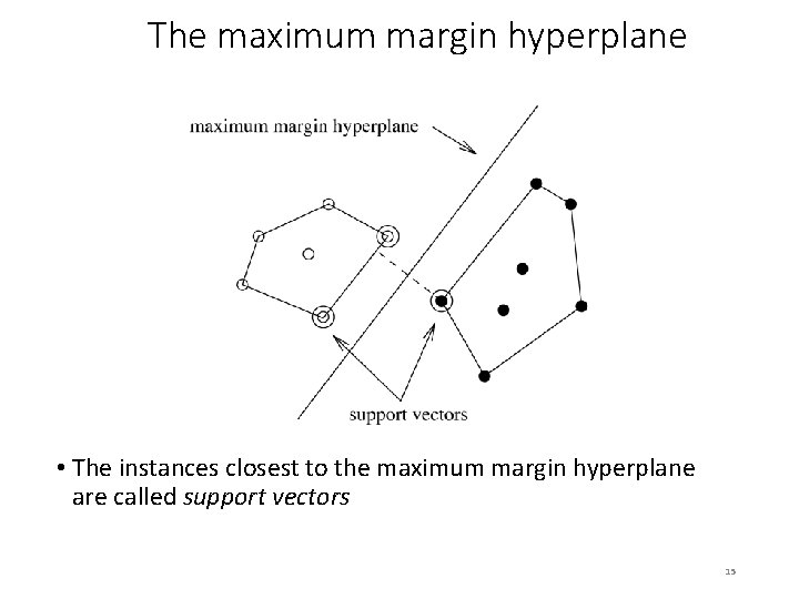
The maximum margin hyperplane • The instances closest to the maximum margin hyperplane are called support vectors 15

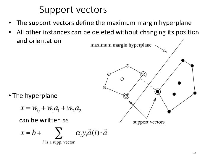
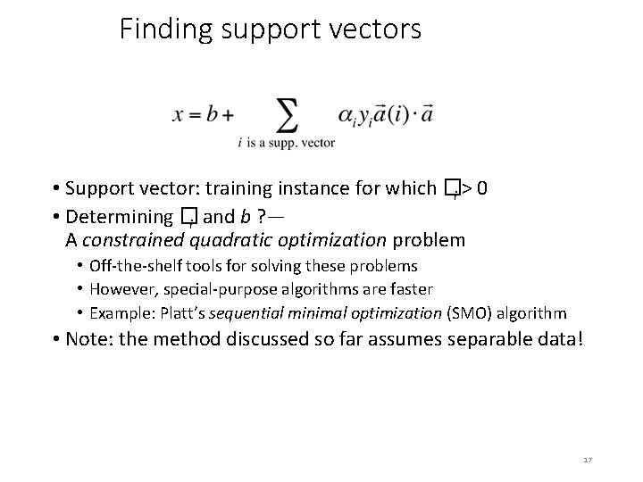
Support vectors • The support vectors define the maximum margin hyperplane • All other instances can be deleted without changing its position and orientation • The hyperplane can be written as 16

Finding support vectors • Support vector: training instance for which �i > 0 • Determining �i and b ? — A constrained quadratic optimization problem • Off-the-shelf tools for solving these problems • However, special-purpose algorithms are faster • Example: Platt’s sequential minimal optimization (SMO) algorithm • Note: the method discussed so far assumes separable data! 17

Nonlinear SVMs • We can create a nonlinear classifier by creating new “pseudo” attributes from the original attributes in the data • “Pseudo” attributes represent attribute combinations • E. g. : all polynomials of degree 2 that can be formed from the original attributes • We can learn a linear SVM from this extended data • The linear SVM in the extended space is a non-linear classifier in the original attribute space • Overfitting often not a significant problem with this approach because the maximum margin hyperplane is stable • There are often comparatively few support vectors relative to the size of the training set • Computation time still an issue • Each time the dot product is computed, all the “pseudo attributes” must be included 18

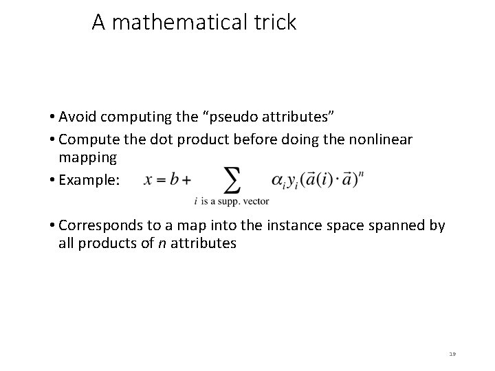
A mathematical trick • Avoid computing the “pseudo attributes” • Compute the dot product before doing the nonlinear mapping • Example: • Corresponds to a map into the instance spanned by all products of n attributes 19

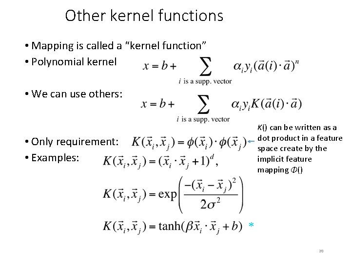
Other kernel functions • Mapping is called a “kernel function” • Polynomial kernel • We can use others: K() can be written as a dot product in a feature space create by the implicit feature mapping Φ() • Only requirement: • Examples: * 20

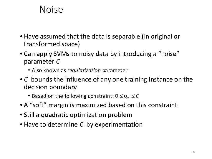
Noise • Have assumed that the data is separable (in original or transformed space) • Can apply SVMs to noisy data by introducing a “noise” parameter C • Also known as regularization parameter • C bounds the influence of any one training instance on the decision boundary • Based on the following constraint: 0 i C • A “soft” margin is maximized based on this constraint • Still a quadratic optimization problem • Have to determine C by experimentation 21

Sparse data • SVM algorithms speed up dramatically if the data is sparse (i. e. , many values are 0) • Why? Because they compute lots and lots of dot products • Sparse data can compute dot products very efficiently • Iterate only over non-zero values • SVMs can process sparse datasets with 10, 000 s of attributes 22

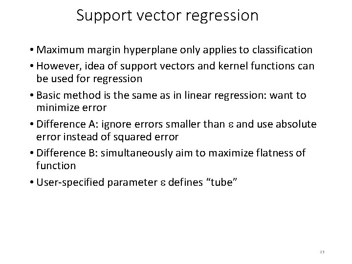
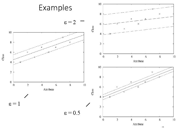
Support vector regression • Maximum margin hyperplane only applies to classification • However, idea of support vectors and kernel functions can be used for regression • Basic method is the same as in linear regression: want to minimize error • Difference A: ignore errors smaller than e and use absolute error instead of squared error • Difference B: simultaneously aim to maximize flatness of function • User-specified parameter e defines “tube” 23

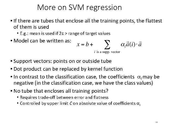
More on SVM regression • If there are tubes that enclose all the training points, the flattest of them is used • E. g. : mean is used if 2 e > range of target values • Model can be written as: • Support vectors: points on or outside tube • Dot product can be replaced by kernel function • In contrast to the classification case, the coefficients i may be negative (in the classification case, we have the class values) • No tube that encloses all training points? • Requires trade-off between error and flatness • Controlled by upper limit C on absolute value of coefficients i 24

Examples e=2 e=1 e = 0. 5 25

Kernel Ridge Regression • For classic linear regression using squared loss, only simple matrix operations are needed to find the parameters • This is not the case for support vector regression because a different loss function is used • Requires use of numeric optimization technique such as sequential minimal optimization • Can we combine the power of the kernel trick with the simplicity of standard least-squares regression? • Yes! This yields kernel ridge regression 26

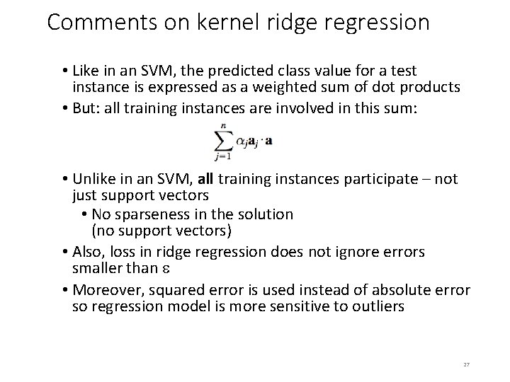
Comments on kernel ridge regression • Like in an SVM, the predicted class value for a test instance is expressed as a weighted sum of dot products • But: all training instances are involved in this sum: • Unlike in an SVM, all training instances participate – not just support vectors • No sparseness in the solution (no support vectors) • Also, loss in ridge regression does not ignore errors smaller than e • Moreover, squared error is used instead of absolute error so regression model is more sensitive to outliers 27

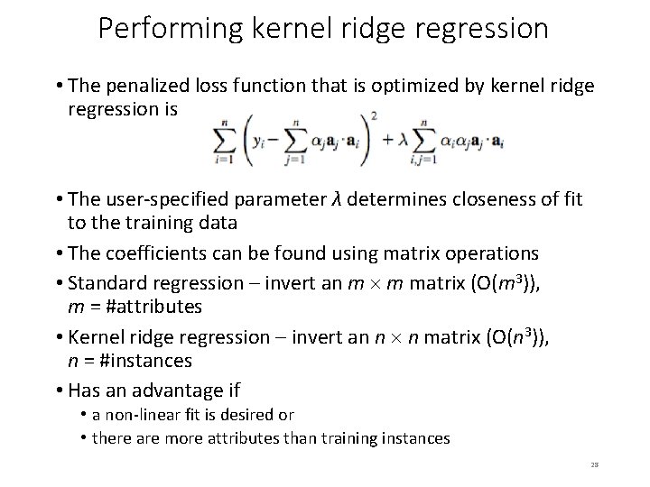
Performing kernel ridge regression • The penalized loss function that is optimized by kernel ridge regression is • The user-specified parameter λ determines closeness of fit to the training data • The coefficients can be found using matrix operations • Standard regression – invert an m m matrix (O(m 3)), m = #attributes • Kernel ridge regression – invert an n n matrix (O(n 3)), n = #instances • Has an advantage if • a non-linear fit is desired or • there are more attributes than training instances 28

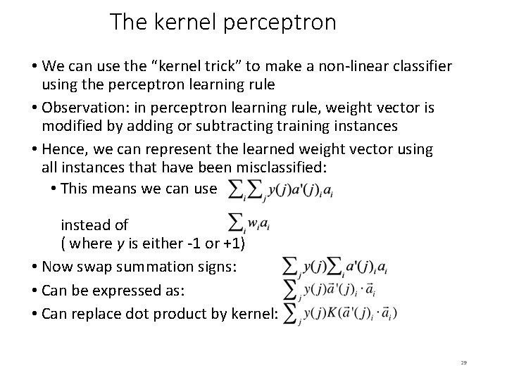
The kernel perceptron • We can use the “kernel trick” to make a non-linear classifier using the perceptron learning rule • Observation: in perceptron learning rule, weight vector is modified by adding or subtracting training instances • Hence, we can represent the learned weight vector using all instances that have been misclassified: • This means we can use instead of ( where y is either -1 or +1) • Now swap summation signs: • Can be expressed as: • Can replace dot product by kernel: 29

Comments on kernel perceptron • Finds separating hyperplane in space created by kernel function (if it exists) • But: doesn't find maximum-margin hyperplane • Easy to implement, supports incremental learning • Perceptron can be made more stable by using all weight vectors encountered during learning, not just the last one (yields the voted perceptron) • Weight vectors vote on prediction (vote based on number of successful classifications sinception) 30

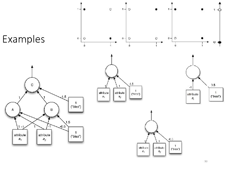
Multilayer perceptrons • Using kernels is only one way to build nonlinear classifier based on perceptrons • Can create network of perceptrons to approximate arbitrary target concepts • A multilayer perceptron is an example of an artificial neural network build from perceptrons • Consists of: input layer, hidden layer(s), and output layer • Structure of MLP is usually found by experimentation • Parameters can be found using backpropagation 31

Examples 32

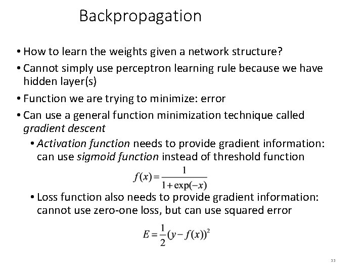
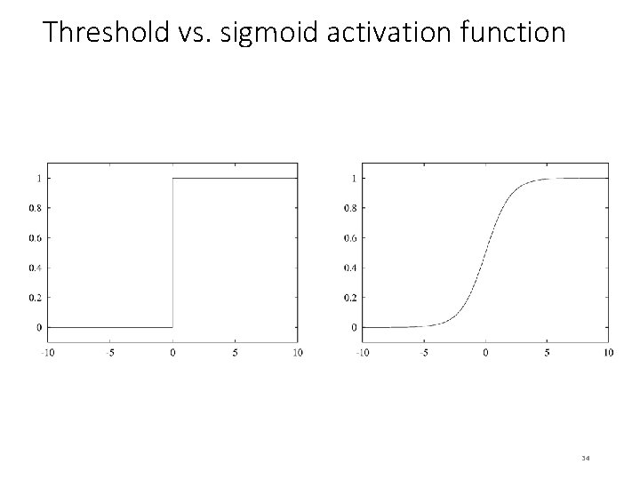
Backpropagation • How to learn the weights given a network structure? • Cannot simply use perceptron learning rule because we have hidden layer(s) • Function we are trying to minimize: error • Can use a general function minimization technique called gradient descent • Activation function needs to provide gradient information: can use sigmoid function instead of threshold function • Loss function also needs to provide gradient information: cannot use zero-one loss, but can use squared error 33

Threshold vs. sigmoid activation function 34

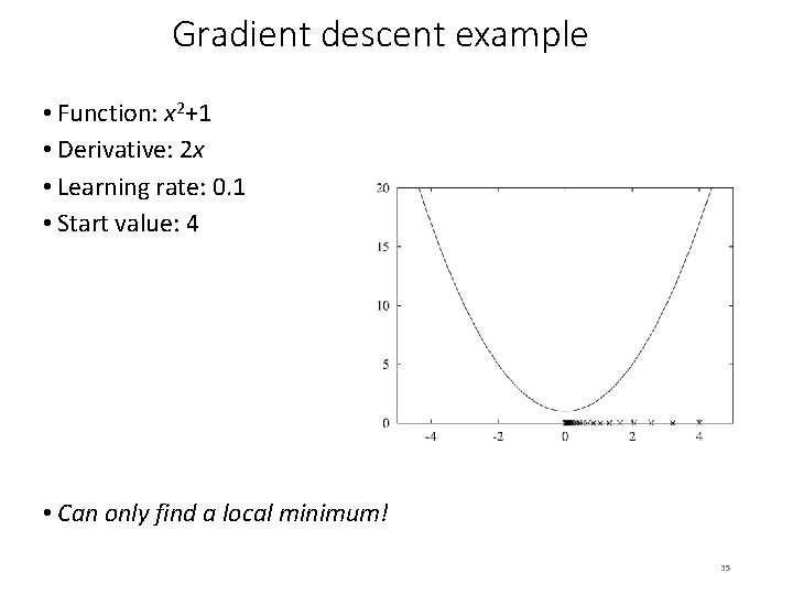
Gradient descent example • Function: x 2+1 • Derivative: 2 x • Learning rate: 0. 1 • Start value: 4 • Can only find a local minimum! 35

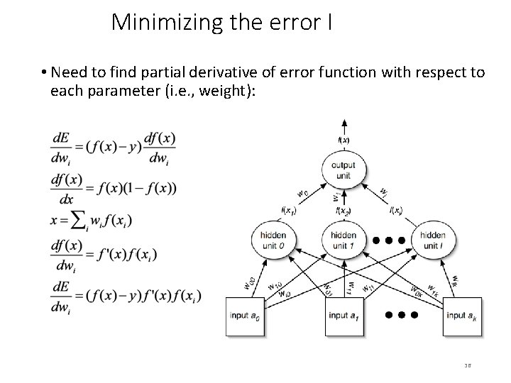
Minimizing the error I • Need to find partial derivative of error function with respect to each parameter (i. e. , weight): 36

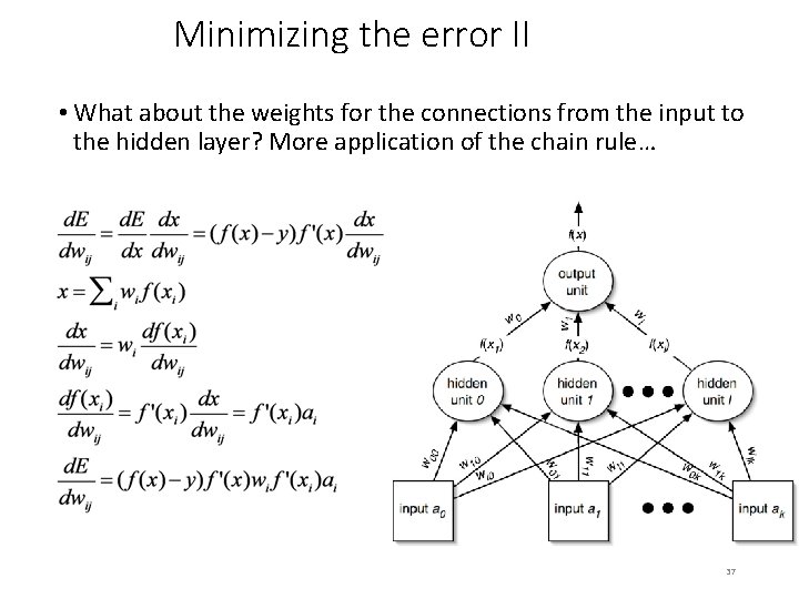
Minimizing the error II • What about the weights for the connections from the input to the hidden layer? More application of the chain rule… 37

Remarks • The same process works for multiple hidden layers and multiple output units (e. g. , for multiple classes) • Can update weights after all training instances have been processed or incrementally: • batch learning vs. stochastic backpropagation • Weights are initialized to small random values • How to avoid overfitting? • Early stopping: use validation set to check when to stop • Weight decay: add penalty term to error function • How to speed up learning? • Momentum: re-use proportion of old weight change • Use optimization method that employs 2 nd derivative 38

Radial basis function networks • RBF network: another type of feedforward network, with two layers (plus the input layer) • Hidden units represent points in instance space and activation depends on distance to these points • To this end, distance is converted into a similarity score using a Gaussian activation function • Width of Gaussian may be different for each hidden unit • Points of equal activation of units in hidden layer form hypersphere (or hyperellipsoid) as opposed to hyperplane • Output layer is the same as in a multi-layer perceptron 39

Learning RBF networks • Parameters to be learned: centers and widths of the RBFs + weights in output layer • Can learn the two sets of parameters independently and still get fairly accurate models • E. g. : clusters from k-means can be used to form basis functions • Linear model for output layer can be based on fixed RBFs found using clustering, which makes learning very efficient • However, for best accuracy it is best to train the entire network in a fully supervised manner • Can use the same methods that are used for training multilayer perceptrons • Disadvantage of standard RBF networks: no built-in attribute weighting based on relevance • But: can introduce attribute weights into the distance function • RBF networks are related to RBF SVMs, which have a basis function centered on each support vector 40

Stochastic gradient descent • We have seen gradient descent + stochastic gradient descent for learning weights in a neural network • Gradient descent is a general-purpose optimization technique • Can be applied whenever the objective function is differentiable • Actually, can be used even when the objective function is not completely differentiable! • This based on the concept of subgradients, which we will not get into here • One application: learning linear models – e. g. linear SVMs or logistic regression • Very fast, simple method for learning from large datasets 41

Stochastic gradient descent cont. • Learning linear models using gradient descent is easier than optimizing non-linear neural networks • Objective function has a single global minimum rather than several local minima • Stochastic gradient descent is fast, uses little memory and is suitable for incremental online learning • Let us look at how to apply stochastic gradient descent to learn a linear support vector machine 42

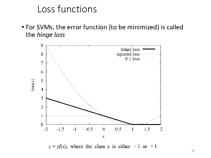
Loss functions • For SVMs, the error function (to be minimized) is called the hinge loss 43

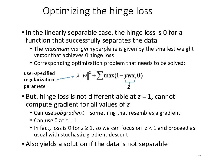
Optimizing the hinge loss • In the linearly separable case, the hinge loss is 0 for a function that successfully separates the data • The maximum margin hyperplane is given by the smallest weight vector that achieves 0 hinge loss • Corresponding optimization problem that needs to be solved: user-specified regularization parameter z • But: hinge loss is not differentiable at z = 1; cannot compute gradient for all values of z • Can use subgradient – something that resembles a gradient • Can use 0 at z = 1 • In fact, loss is 0 for z 1, so we can focus on z 1 and proceed as usual with stochastic gradient descent • Also yields a solution if the data is not separable 44

Discussion and Bibliographic Notes • SVMs stem from statistical learning theory (Vapnik 1999) • A good starting point for exploration is a tutorial by Burges (1998) • Soft-margin SVMs were discussed by Cortes and Vapnik (1995) • Tutorial on support vector regression: Smola and Schölkopf (2004) • Schölkopf et al. (1999) present support vector regression with just one parameter instead of two (C and ε) • Fletcher (1987) covers constrained quadratic optimization • The SMO algorithm for training SVMs is due to Platt (1998) • Ridge regression was introduced by Hoerl and Kennard (1970) • Hastie et al. (2009) give a good description of kernel ridge regression • Kernel ridge regression is equivalent to Gaussian process regression, a Bayesian approach that also provides estimates of uncertainty 45

Discussion and Bibliographic Notes • The kernel perceptron is due to Freund and Schapire (1999) • Cristianini and Shawe-Taylor (2000) provide an introduction to support vector machines and kernel-based methods • Shawe-Taylor and Cristianini (2004) and Schölkopf and Smola (2002) cover kernel-based learning in detail • Bishop (1995) provides an excellent introduction to both multilayer perceptrons and RBF networks • Kivinen et al. (2002), Zhang (2004) and Shalev-Shwartz et al. (2007) explore gradient methods for SVMs • Kivinen et al. and Shalev-Shwartz et al. provide heuristics for setting the learning rate for gradient descent 46

Numeric Prediction with Local Linear Models 47

Numeric prediction (aka regression) • Counterparts exist for all classification schemes previously discussed • Decision trees, rule learners, SVMs, etc. • (Almost) all classification schemes can be applied to regression problems using discretization: • Discretize the class into intervals • Predict weighted average of interval representatives (e. g. , midpoints) • Weight according to class probabilities • We will cover a couple of approaches to regression that are based on building local linear models • Model trees (+ a rule learning algorithm based on them) and locally weighted linear regression 48

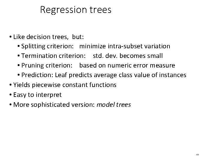
Regression trees • Like decision trees, but: • Splitting criterion: minimize intra-subset variation • Termination criterion: std. dev. becomes small • Pruning criterion: based on numeric error measure • Prediction: Leaf predicts average class value of instances • Yields piecewise constant functions • Easy to interpret • More sophisticated version: model trees 49

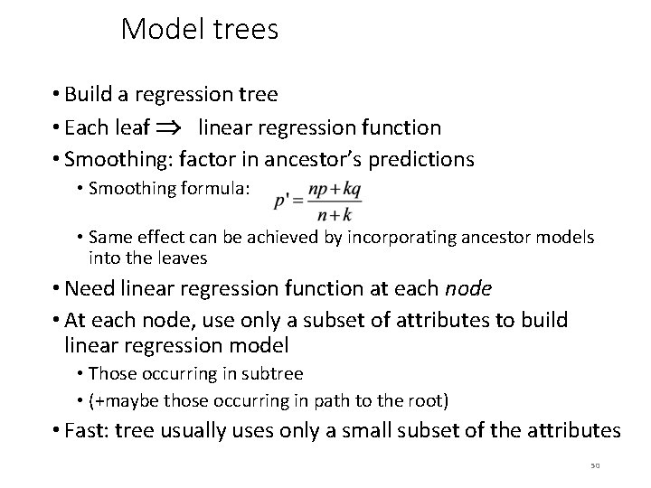
Model trees • Build a regression tree • Each leaf linear regression function • Smoothing: factor in ancestor’s predictions • Smoothing formula: • Same effect can be achieved by incorporating ancestor models into the leaves • Need linear regression function at each node • At each node, use only a subset of attributes to build linear regression model • Those occurring in subtree • (+maybe those occurring in path to the root) • Fast: tree usually uses only a small subset of the attributes 50

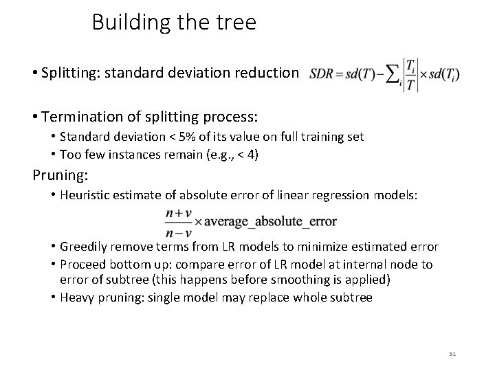
Building the tree • Splitting: standard deviation reduction • Termination of splitting process: • Standard deviation < 5% of its value on full training set • Too few instances remain (e. g. , < 4) Pruning: • Heuristic estimate of absolute error of linear regression models: • Greedily remove terms from LR models to minimize estimated error • Proceed bottom up: compare error of LR model at internal node to error of subtree (this happens before smoothing is applied) • Heavy pruning: single model may replace whole subtree 51

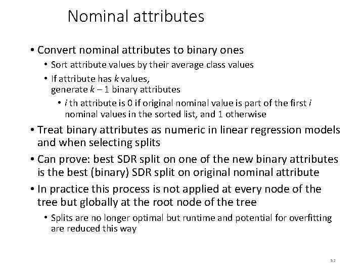
Nominal attributes • Convert nominal attributes to binary ones • Sort attribute values by their average class values • If attribute has k values, generate k – 1 binary attributes • i th attribute is 0 if original nominal value is part of the first i nominal values in the sorted list, and 1 otherwise • Treat binary attributes as numeric in linear regression models and when selecting splits • Can prove: best SDR split on one of the new binary attributes is the best (binary) SDR split on original nominal attribute • In practice this process is not applied at every node of the tree but globally at the root node of the tree • Splits are no longer optimal but runtime and potential for overfitting are reduced this way 52

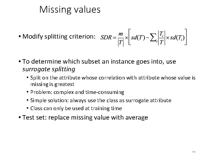
Missing values • Modify splitting criterion: • To determine which subset an instance goes into, use surrogate splitting • Split on the attribute whose correlation with attribute whose value is missing is greatest • Problem: complex and time-consuming • Simple solution: always use the class as surrogate attribute • Class can only be used at training time • Test set: replace missing value with average 53

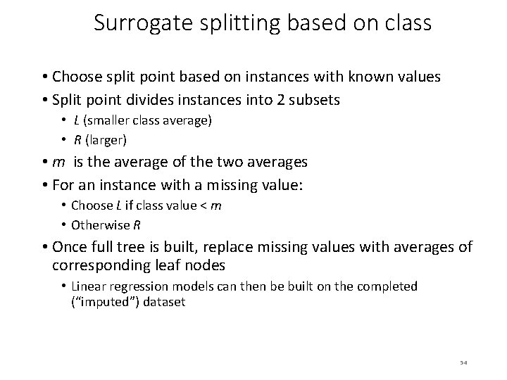
Surrogate splitting based on class • Choose split point based on instances with known values • Split point divides instances into 2 subsets • L (smaller class average) • R (larger) • m is the average of the two averages • For an instance with a missing value: • Choose L if class value < m • Otherwise R • Once full tree is built, replace missing values with averages of corresponding leaf nodes • Linear regression models can then be built on the completed (“imputed”) dataset 54

Pseudo-code for M 5' • Let us consider the pseudo code for the model tree inducer M 5’ • Four methods: • • Main method: Make. Model. Tree Method for splitting: split Method for pruning: prune Method that computes error: subtree. Error • We will briefly look at each method in turn • We will assume that the linear regression method performs attribute subset selection based on error (discussed previously) • Nominal attributes are replaced globally at the root node 55

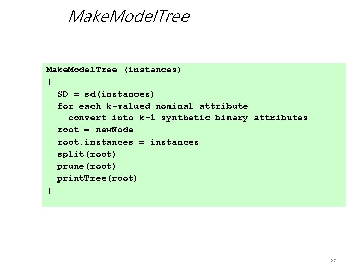
Make. Model. Tree (instances) { SD = sd(instances) for each k-valued nominal attribute convert into k-1 synthetic binary attributes root = new. Node root. instances = instances split(root) prune(root) print. Tree(root) } 56

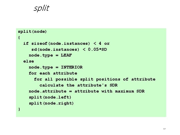
split(node) { if sizeof(node. instances) < 4 or sd(node. instances) < 0. 05*SD node. type = LEAF else node. type = INTERIOR for each attribute for all possible split positions of attribute calculate the attribute's SDR node. attribute = attribute with maximum SDR split(node. left) split(node. right) } 57

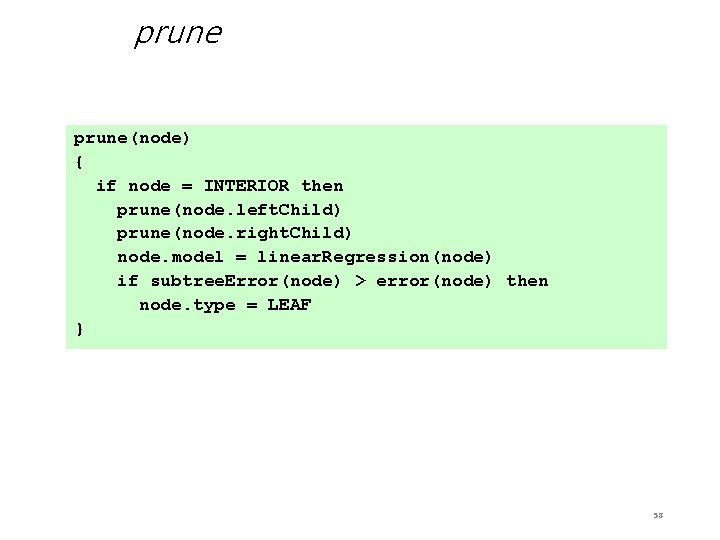
prune(node) { if node = INTERIOR then prune(node. left. Child) prune(node. right. Child) node. model = linear. Regression(node) if subtree. Error(node) > error(node) then node. type = LEAF } 58

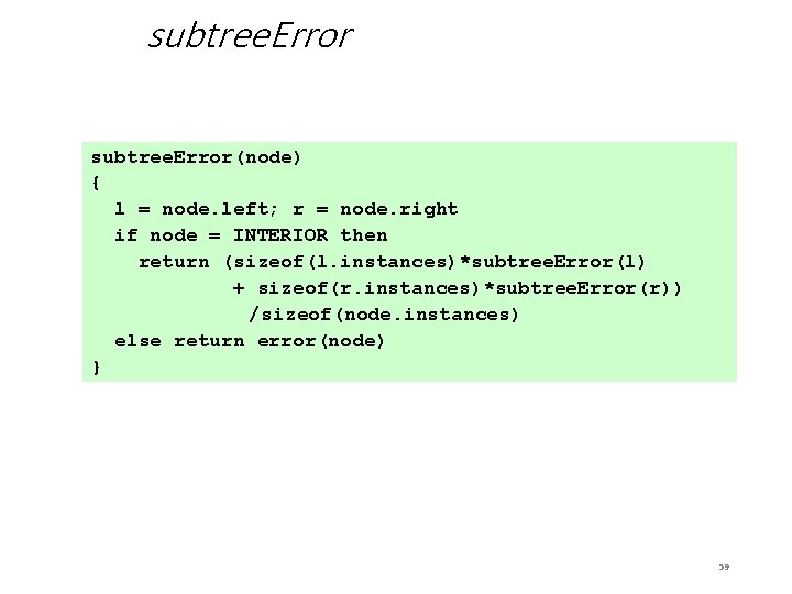
subtree. Error(node) { l = node. left; r = node. right if node = INTERIOR then return (sizeof(l. instances)*subtree. Error(l) + sizeof(r. instances)*subtree. Error(r)) /sizeof(node. instances) else return error(node) } 59

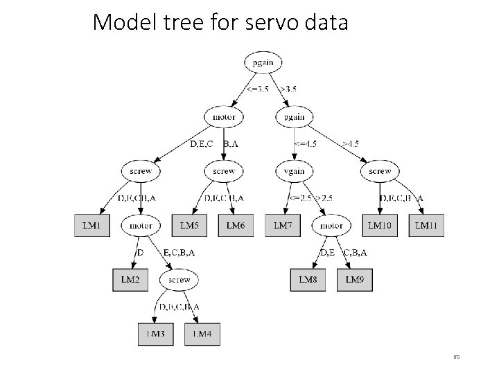
Model tree for servo data 60

Rules from model trees • PART algorithm generates classification rules by building partial decision trees • Can use the same method to build rule sets for regression • Use model trees instead of decision trees • Use variance instead of entropy to choose node to expand when building a partial tree • Rules that are generated will have linear models on righthand side • Caveat: using smoothed trees may not be appropriate due to the separate-and-conquer strategy used in rule learning • Empirical evidence shows that smoothing does not help • Full trees can be used instead of partial trees at the expense of runtime 61

Locally weighted regression • Locally weighted regression is a numeric prediction method that combines • instance-based learning • linear regression • It is a “lazy” learning method: • Computes new regression function for each test instance at prediction time • Works incrementally • Weights training instances • according to distance to test instance • builds linear regression model from weighted data • requires weighted version of linear regression (straightforward) • Advantage: nonlinear approximation • Slow if implemented using brute-force search; however, fast data structures can be used for the nearest-neighbor search 62

Design decisions • Weighting functions: • • Inverse Euclidean distance Gaussian kernel applied to Euclidean distance Triangular kernel used the same way etc. • Empirically, performance does not appear to depend much on the weighting method that is used • Ideally, weighting function has bounded support so that most training instances receive weight 0 and can be ignored • Smoothing parameter is used to scale the distance function for computation of the weights • Multiply distance by inverse of this parameter • Possible choice: distance to the kth nearest training instance (renders choice of smoothing parameter data dependent) 63

Discussion and Bibliographic Notes • Regression trees were introduced in the “classification and regression trees”, or CART system (Breiman et al. , 1984) • The method of handling nominal attributes and the surrogate device for dealing with missing values were included in CART • M 5 model trees were first described by Quinlan (1992) • The M 5’ version is given by Wang and Witten (1997) • Using model trees (although not partial trees) for generating rule sets has been explored by Hall et al. (1999) • There are many variations of locally weighted learning. • Statisticians have considered using locally quadratic models • They have applied locally weighted logistic regression to classification • Frank et al. (2003) evaluated the use of locally weighted learning in conjunction with Naïve Bayes • Atkeson et al. (1997) provide a survey on locally weighted learning 64