Data Mining Practical Machine Learning Tools and Techniques

Data Mining Practical Machine Learning Tools and Techniques Slides for Chapter 4, Algorithms: the basic methods of Data Mining by I. H. Witten, E. Frank, M. A. Hall and C. J. Pal

Algorithms: The basic methods • • • Inferring rudimentary rules Simple probabilistic modeling Constructing decision trees Constructing rules Association rule learning Linear models Instance-based learning Clustering Multi-instance learning 2

Simplicity first • • Simple algorithms often work very well! There are many kinds of simple structure, e. g. : • • • One attribute does all the work All attributes contribute equally & independently Logical structure with a few attributes suitable for tree A set of simple logical rules Relationships between groups of attributes A weighted linear combination of the attributes Strong neighborhood relationships based on distance Clusters of data in unlabeled data Bags of instances that can be aggregated Success of method depends on the domain 3

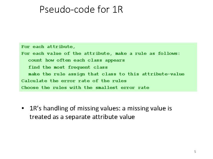
Inferring rudimentary rules • 1 R rule learner: learns a 1 -level decision tree • A set of rules that all test one particular attribute that has been identified as the one that yields the lowest classification error • Basic version for finding the rule set from a given training set (assumes nominal attributes): • For each attribute • Make one branch for each value of the attribute • To each branch, assign the most frequent class value of the instances pertaining to that branch • Error rate: proportion of instances that do not belong to the majority class of their corresponding branch • Choose attribute with lowest error rate 4

Pseudo-code for 1 R For each attribute, For each value of the attribute, make a rule as follows: count how often each class appears find the most frequent class make the rule assign that class to this attribute-value Calculate the error rate of the rules Choose the rules with the smallest error rate • 1 R’s handling of missing values: a missing value is treated as a separate attribute value 5

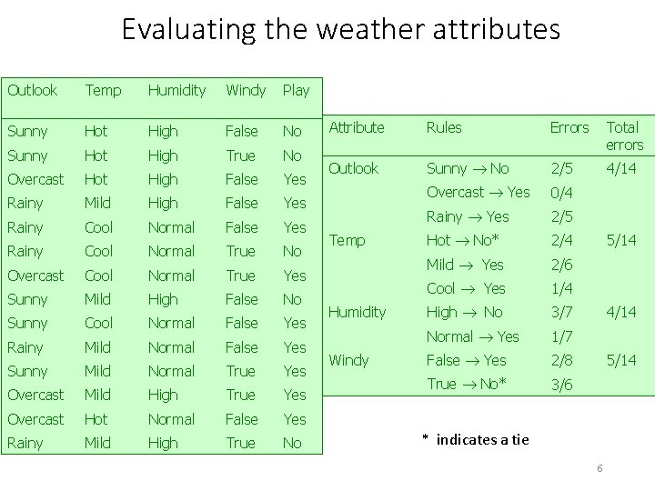
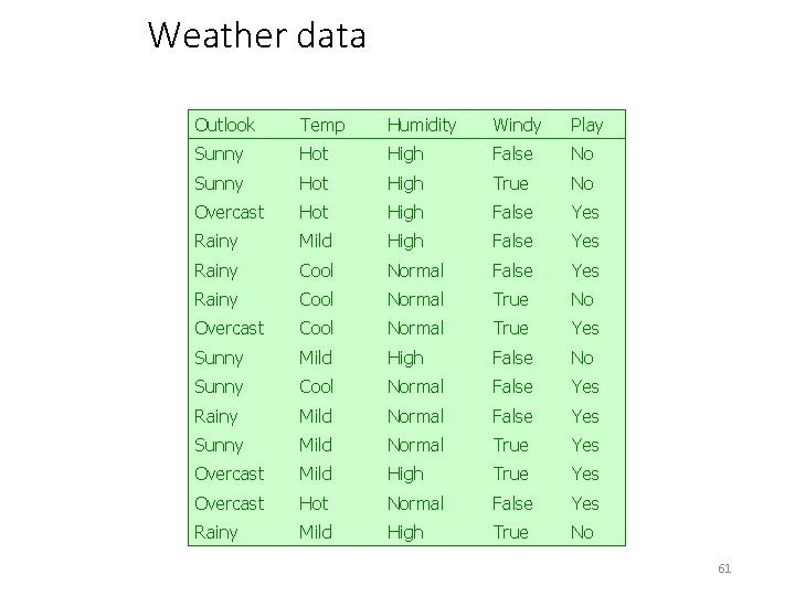
Evaluating the weather attributes Outlook Temp Humidity Windy Play Sunny Hot High False No Sunny Hot High True No Overcast Hot High False Yes Rainy Mild High False Yes Rainy Cool Normal True No Overcast Cool Normal True Yes Sunny Mild High False No Sunny Cool Normal False Yes Rainy Mild Normal False Yes Sunny Mild Normal True Yes Overcast Mild High True Yes Overcast Hot Normal False Yes Rainy Mild High True No Attribute Rules Errors Total errors Outlook Sunny No 2/5 4/14 Overcast Yes 0/4 Rainy Yes 2/5 Hot No* 2/4 Mild Yes 2/6 Cool Yes 1/4 High No 3/7 Normal Yes 1/7 False Yes 2/8 True No* 3/6 Temp Humidity Windy 5/14 4/14 5/14 * indicates a tie 6

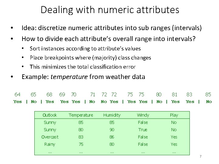
Dealing with numeric attributes • • Idea: discretize numeric attributes into sub ranges (intervals) How to divide each attribute’s overall range into intervals? • Sort instances according to attribute’s values • Place breakpoints where (majority) class changes • This minimizes the total classification error • Example: temperature from weather data 64 65 68 Yes | No | Yes 69 70 71 Yes | No 72 72 75 75 80 81 No Yes | No | Yes Outlook Temperature Humidity Windy Play Sunny 85 85 False No Sunny 80 90 True No Overcast 83 86 False Yes Rainy 75 80 False Yes … … … 83 Yes | 7 85 No

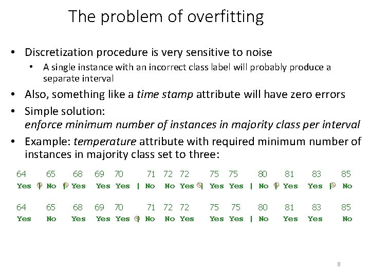
The problem of overfitting • Discretization procedure is very sensitive to noise • A single instance with an incorrect class label will probably produce a separate interval • Also, something like a time stamp attribute will have zero errors • Simple solution: enforce minimum number of instances in majority class per interval • Example: temperature attribute with required minimum number of instances in majority class set to three: 64 65 68 Yes | No | Yes 69 70 71 72 72 75 75 80 81 Yes | No No Yes | No | Yes 83 Yes | 85 No 64 Yes 69 70 71 72 72 Yes | No No Yes 83 Yes 85 No 68 Yes 75 75 80 Yes | No 81 Yes 8

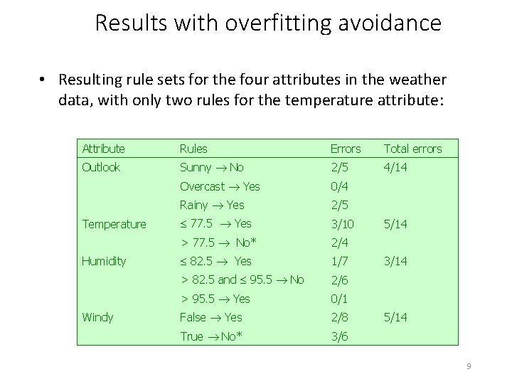
Results with overfitting avoidance • Resulting rule sets for the four attributes in the weather data, with only two rules for the temperature attribute: Attribute Rules Errors Total errors Outlook Sunny No 2/5 4/14 Overcast Yes 0/4 Rainy Yes 2/5 77. 5 Yes 3/10 > 77. 5 No* 2/4 82. 5 Yes 1/7 > 82. 5 and 95. 5 No 2/6 > 95. 5 Yes 0/1 False Yes 2/8 True No* 3/6 Temperature Humidity Windy 5/14 3/14 5/14 9

Discussion of 1 R • 1 R was described in a paper by Holte (1993): Very Simple Classification Rules Perform Well on Most Commonly Used Datasets Robert C. Holte, Computer Science Department, University of Ottawa • Contains an experimental evaluation on 16 datasets (using crossvalidation to estimate classification accuracy on fresh data) • Required minimum number of instances in majority class was set to 6 after some experimentation • 1 R’s simple rules performed not much worse than much more complex decision trees • Lesson: simplicity first can pay off on practical datasets • Note that 1 R does not perform as well on more recent, more sophisticated benchmark datasets 10

Simple probabilistic modeling • “Opposite” of 1 R: use all the attributes • Two assumptions: Attributes are • equally important • statistically independent (given the class value) • This means knowing the value of one attribute tells us nothing about the value of another takes on (if the class is known) • Independence assumption is almost never correct! • But … this scheme often works surprisingly well in practice • The scheme is easy to implement in a program and very fast • It is known as naïve Bayes 11

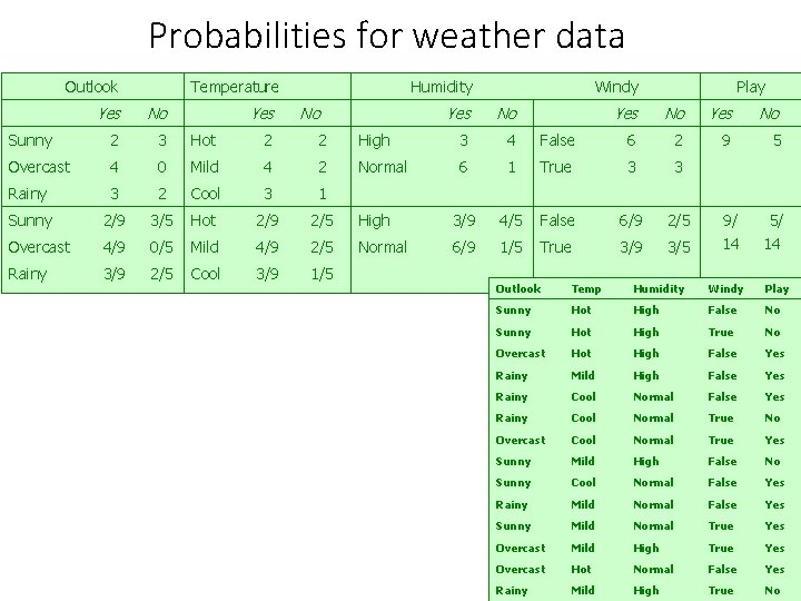
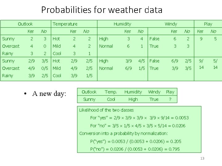
Probabilities for weather data Outlook Temperature Yes Humidity Yes No No Sunny 2 3 Hot 2 2 Overcast 4 0 Mild 4 2 Rainy 3 2 Cool 3 1 Sunny 2/9 3/5 Hot 2/9 2/5 Overcast 4/9 0/5 Mild 4/9 2/5 Rainy 3/9 2/5 Cool 3/9 1/5 Windy Yes No High 3 4 Normal 6 High Normal Play Yes No False 6 2 9 5 1 True 3 3 3/9 4/5 False 6/9 2/5 6/9 1/5 True 3/9 3/5 9/ 14 5/ 14 Outlook Temp Humidity Windy Play Sunny Hot High False No Sunny Hot High True No Overcast Hot High False Yes Rainy Mild High False Yes Rainy Cool Normal True No Overcast Cool Normal True Yes Sunny Mild High False No Sunny Cool Normal False Yes Rainy Mild Normal False Yes Sunny Mild Normal True Yes Overcast Mild High True Yes Overcast Hot Normal False 12 Yes Rainy Mild High True No

Probabilities for weather data Outlook Temperature Yes Humidity Yes No Sunny 2 3 Hot 2 2 Overcast 4 0 Mild 4 2 Rainy 3 2 Cool 3 1 Sunny 2/9 3/5 Hot 2/9 2/5 Overcast 4/9 0/5 Mild 4/9 2/5 Rainy 3/9 2/5 Cool 3/9 1/5 • A new day: No Windy Yes No High 3 4 Normal 6 High Normal Play Yes No False 6 2 9 5 1 True 3 3 3/9 4/5 False 6/9 2/5 6/9 1/5 True 3/9 3/5 9/ 14 5/ 14 Outlook Temp. Humidity Windy Play Sunny Cool High True ? Likelihood of the two classes For “yes” = 2/9 3/9 9/14 = 0. 0053 For “no” = 3/5 1/5 4/5 3/5 5/14 = 0. 0206 Conversion into a probability by normalization: P(“yes”) = 0. 0053 / (0. 0053 + 0. 0206) = 0. 205 P(“no”) = 0. 0206 / (0. 0053 + 0. 0206) = 0. 795 13

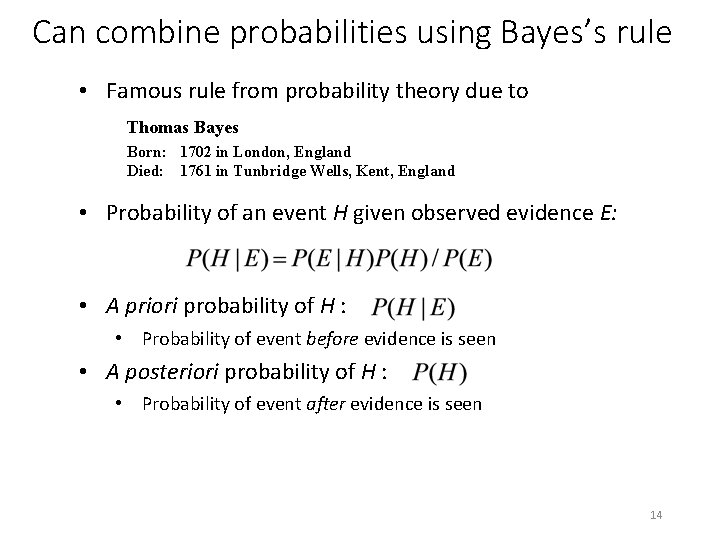
Can combine probabilities using Bayes’s rule • Famous rule from probability theory due to Thomas Bayes Born: 1702 in London, England Died: 1761 in Tunbridge Wells, Kent, England • Probability of an event H given observed evidence E: • A priori probability of H : • Probability of event before evidence is seen • A posteriori probability of H : • Probability of event after evidence is seen 14

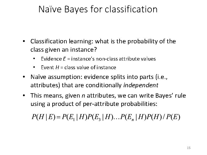
Naïve Bayes for classification • Classification learning: what is the probability of the class given an instance? • Evidence E = instance’s non-class attribute values • Event H = class value of instance • Naïve assumption: evidence splits into parts (i. e. , attributes) that are conditionally independent • This means, given n attributes, we can write Bayes’ rule using a product of per-attribute probabilities: 15

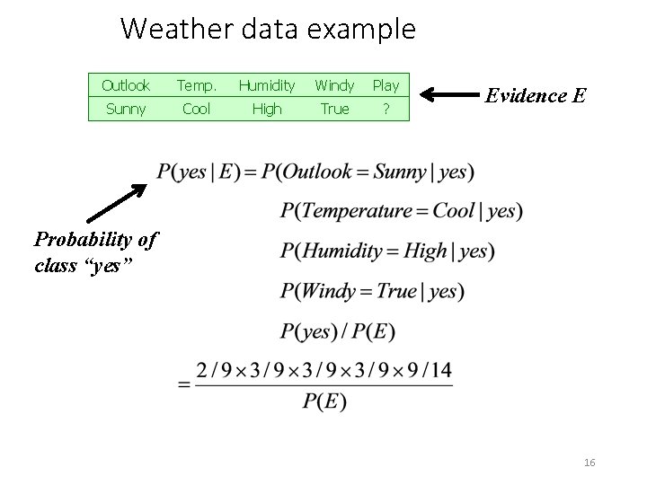
Weather data example Outlook Temp. Humidity Windy Play Sunny Cool High True ? Evidence E Probability of class “yes” 16

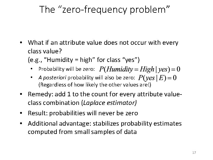
The “zero-frequency problem” • What if an attribute value does not occur with every class value? (e. g. , “Humidity = high” for class “yes”) • Probability will be zero: • A posteriori probability will also be zero: (Regardless of how likely the other values are!) • Remedy: add 1 to the count for every attribute valueclass combination (Laplace estimator) • Result: probabilities will never be zero • Additional advantage: stabilizes probability estimates computed from small samples of data 17

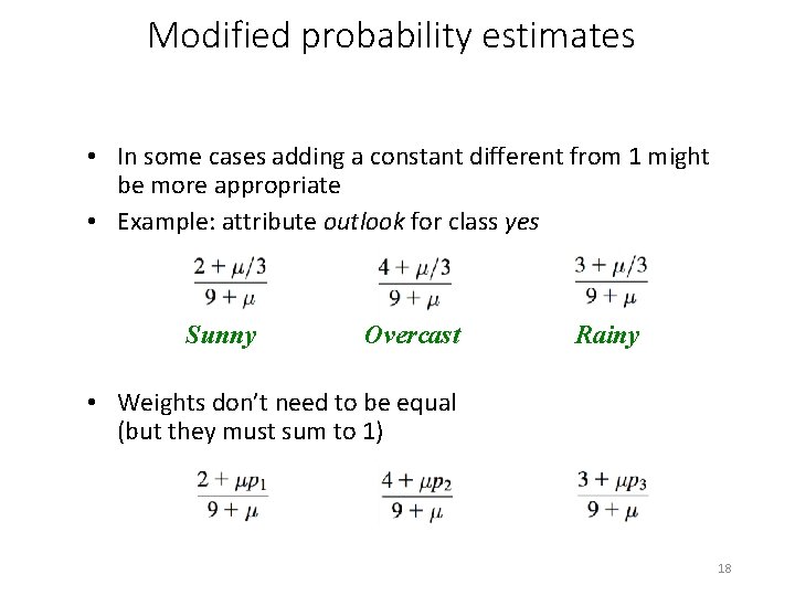
Modified probability estimates • In some cases adding a constant different from 1 might be more appropriate • Example: attribute outlook for class yes Sunny Overcast Rainy • Weights don’t need to be equal (but they must sum to 1) 18

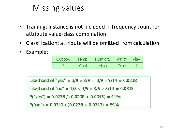
Missing values • Training: instance is not included in frequency count for attribute value-class combination • Classification: attribute will be omitted from calculation • Example: Outlook Temp. Humidity Windy Play ? Cool High True ? Likelihood of “yes” = 3/9 9/14 = 0. 0238 Likelihood of “no” = 1/5 4/5 3/5 5/14 = 0. 0343 P(“yes”) = 0. 0238 / (0. 0238 + 0. 0343) = 41% P(“no”) = 0. 0343 / (0. 0238 + 0. 0343) = 59% 19

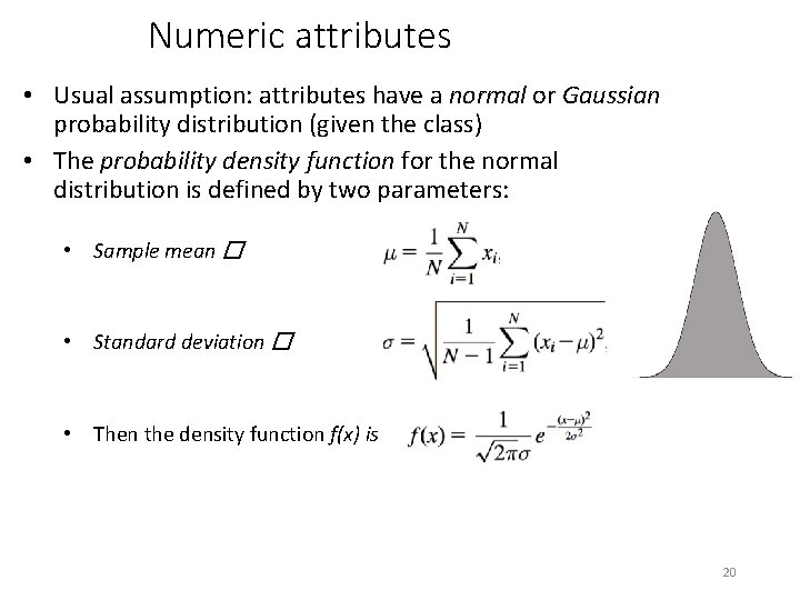
Numeric attributes • Usual assumption: attributes have a normal or Gaussian probability distribution (given the class) • The probability density function for the normal distribution is defined by two parameters: • Sample mean � • Standard deviation � • Then the density function f(x) is 20

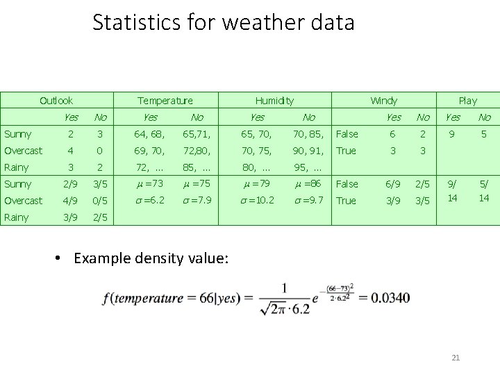
Statistics for weather data Outlook Temperature Humidity Windy Yes No Sunny 2 3 64, 68, 65, 71, 65, 70, 85, Overcast 4 0 69, 70, 72, 80, 70, 75, 90, 91, Rainy 3 2 72, … 85, … 80, … 95, … Sunny 2/9 3/5 =73 =75 =79 Overcast 4/9 0/5 =6. 2 =7. 9 =10. 2 Rainy 3/9 2/5 Play Yes No False 6 2 9 5 True 3 3 =86 False 6/9 2/5 =9. 7 True 3/9 3/5 9/ 14 5/ 14 • Example density value: 21

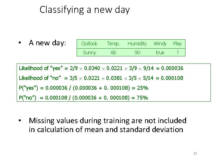
Classifying a new day • A new day: Outlook Temp. Humidity Windy Play Sunny 66 90 true ? Likelihood of “yes” = 2/9 0. 0340 0. 0221 3/9 9/14 = 0. 000036 Likelihood of “no” = 3/5 0. 0221 0. 0381 3/5 5/14 = 0. 000108 P(“yes”) = 0. 000036 / (0. 000036 + 0. 000108) = 25% P(“no”) = 0. 000108 / (0. 000036 + 0. 000108) = 75% • Missing values during training are not included in calculation of mean and standard deviation 22

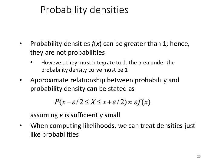
Probability densities • Probability densities f(x) can be greater than 1; hence, they are not probabilities • • • However, they must integrate to 1: the area under the probability density curve must be 1 Approximate relationship between probability and probability density can be stated as assuming ε is sufficiently small When computing likelihoods, we can treat densities just like probabilities 23

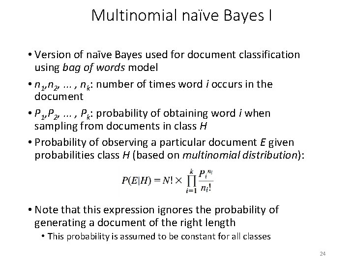
Multinomial naïve Bayes I • Version of naïve Bayes used for document classification using bag of words model • n 1, n 2, . . . , nk: number of times word i occurs in the document • P 1, P 2, . . . , Pk: probability of obtaining word i when sampling from documents in class H • Probability of observing a particular document E given probabilities class H (based on multinomial distribution): • Note that this expression ignores the probability of generating a document of the right length • This probability is assumed to be constant for all classes 24

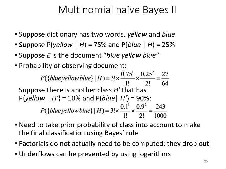
Multinomial naïve Bayes II • Suppose dictionary has two words, yellow and blue • Suppose P(yellow | H) = 75% and P(blue | H) = 25% • Suppose E is the document “blue yellow blue” • Probability of observing document: Suppose there is another class H' that has P(yellow | H’) = 10% and P(blue| H’) = 90%: • Need to take prior probability of class into account to make the final classification using Bayes’ rule • Factorials do not actually need to be computed: they drop out • Underflows can be prevented by using logarithms 25

Naïve Bayes: discussion • Naïve Bayes works surprisingly well even if independence assumption is clearly violated • Why? Because classification does not require accurate probability estimates as long as maximum probability is assigned to the correct class • However: adding too many redundant attributes will cause problems (e. g. , identical attributes) • Note also: many numeric attributes are not normally distributed (kernel density estimators can be used instead) 26

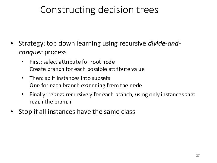
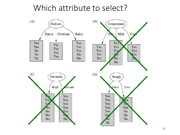
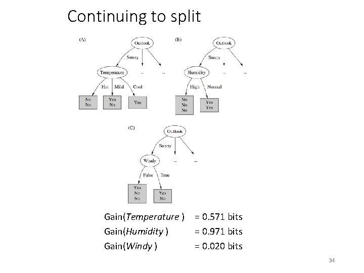
Constructing decision trees • Strategy: top down learning using recursive divide-andconquer process • First: select attribute for root node Create branch for each possible attribute value • Then: split instances into subsets One for each branch extending from the node • Finally: repeat recursively for each branch, using only instances that reach the branch • Stop if all instances have the same class 27

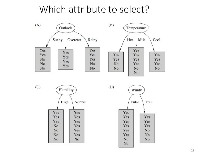
Which attribute to select? 28

Which attribute to select? 29

Criterion for attribute selection • Which is the best attribute? • Want to get the smallest tree • Heuristic: choose the attribute that produces the “purest” nodes • Popular selection criterion: information gain • Information gain increases with the average purity of the subsets • Strategy: amongst attributes available for splitting, choose attribute that gives greatest information gain • Information gain requires measure of impurity • Impurity measure that it uses is the entropy of the class distribution, which is a measure from information theory 30

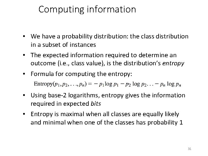
Computing information • We have a probability distribution: the class distribution in a subset of instances • The expected information required to determine an outcome (i. e. , class value), is the distribution’s entropy • Formula for computing the entropy: • Using base-2 logarithms, entropy gives the information required in expected bits • Entropy is maximal when all classes are equally likely and minimal when one of the classes has probability 1 31

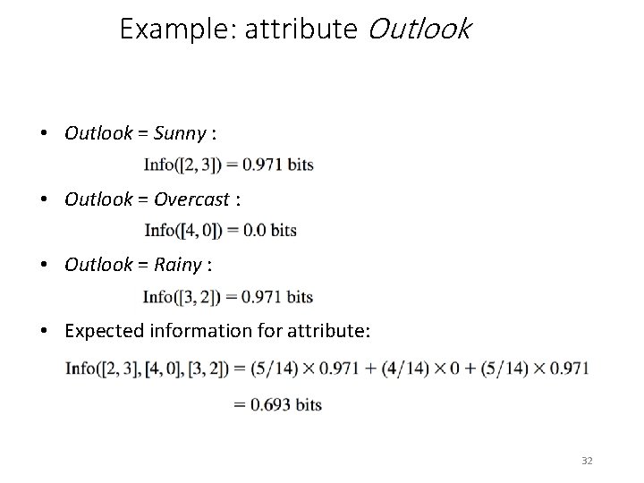
Example: attribute Outlook • Outlook = Sunny : • Outlook = Overcast : • Outlook = Rainy : • Expected information for attribute: 32

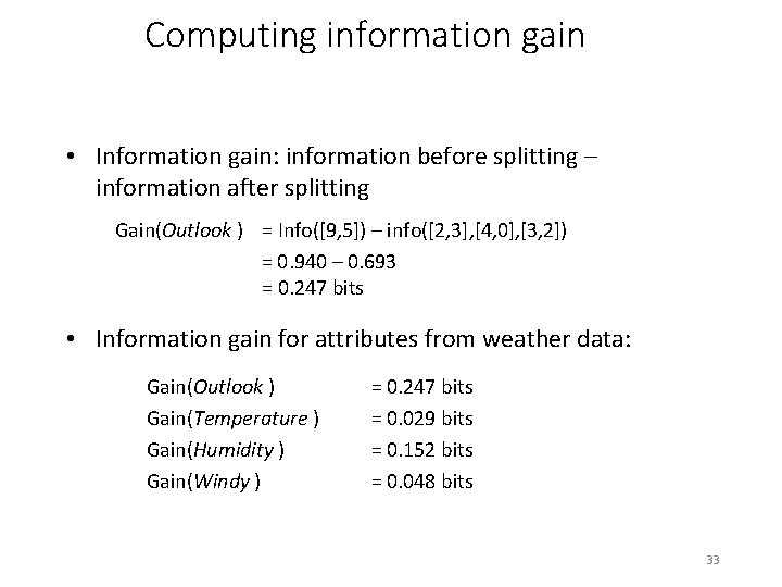
Computing information gain • Information gain: information before splitting – information after splitting Gain(Outlook ) = Info([9, 5]) – info([2, 3], [4, 0], [3, 2]) = 0. 940 – 0. 693 = 0. 247 bits • Information gain for attributes from weather data: Gain(Outlook ) Gain(Temperature ) Gain(Humidity ) Gain(Windy ) = 0. 247 bits = 0. 029 bits = 0. 152 bits = 0. 048 bits 33

Continuing to split Gain(Temperature ) Gain(Humidity ) Gain(Windy ) = 0. 571 bits = 0. 971 bits = 0. 020 bits 34

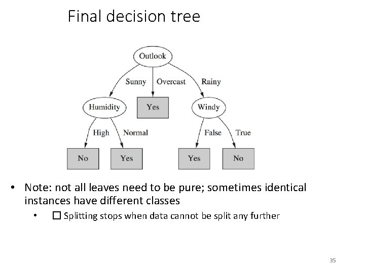
Final decision tree • Note: not all leaves need to be pure; sometimes identical instances have different classes • � Splitting stops when data cannot be split any further 35

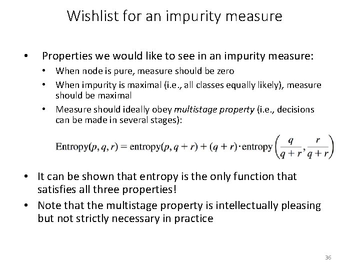
Wishlist for an impurity measure • Properties we would like to see in an impurity measure: • When node is pure, measure should be zero • When impurity is maximal (i. e. , all classes equally likely), measure should be maximal • Measure should ideally obey multistage property (i. e. , decisions can be made in several stages): • It can be shown that entropy is the only function that satisfies all three properties! • Note that the multistage property is intellectually pleasing but not strictly necessary in practice 36

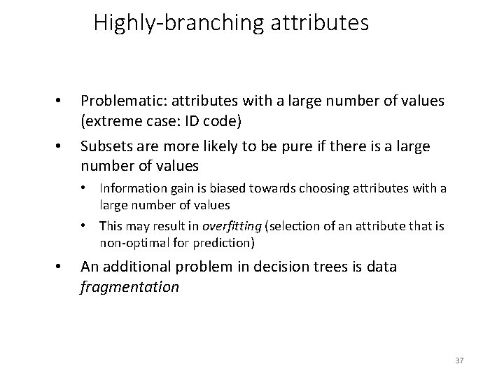
Highly-branching attributes • • Problematic: attributes with a large number of values (extreme case: ID code) Subsets are more likely to be pure if there is a large number of values • Information gain is biased towards choosing attributes with a large number of values • This may result in overfitting (selection of an attribute that is non-optimal for prediction) • An additional problem in decision trees is data fragmentation 37

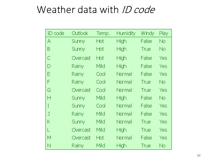
Weather data with ID code Outlook Temp. Humidity Windy Play A Sunny Hot High False No B Sunny Hot High True No C Overcast Hot High False Yes D Rainy Mild High False Yes E Rainy Cool Normal False Yes F Rainy Cool Normal True No G Overcast Cool Normal True Yes H Sunny Mild High False No I Sunny Cool Normal False Yes J Rainy Mild Normal False Yes K Sunny Mild Normal True Yes L Overcast Mild High True Yes M Overcast Hot Normal False Yes N Rainy Mild High True No 38

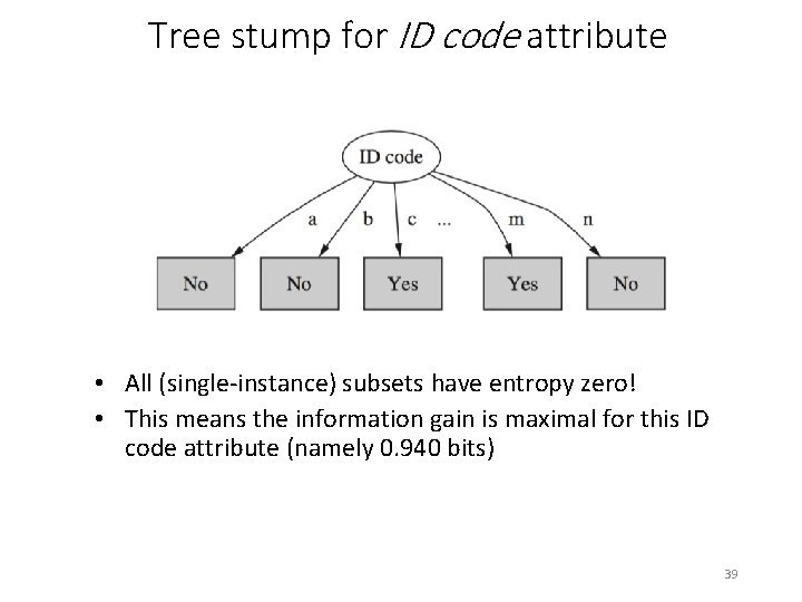
Tree stump for ID code attribute • All (single-instance) subsets have entropy zero! • This means the information gain is maximal for this ID code attribute (namely 0. 940 bits) 39

Gain ratio • Gain ratio is a modification of the information gain that reduces its bias towards attributes with many values • Gain ratio takes number and size of branches into account when choosing an attribute • It corrects the information gain by taking the intrinsic information of a split into account • Intrinsic information: entropy of the distribution of instances into branches • Measures how much info do we need to tell which branch a randomly chosen instance belongs to 40

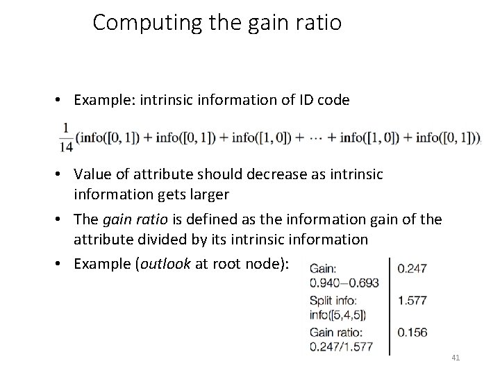
Computing the gain ratio • Example: intrinsic information of ID code • Value of attribute should decrease as intrinsic information gets larger • The gain ratio is defined as the information gain of the attribute divided by its intrinsic information • Example (outlook at root node): 41

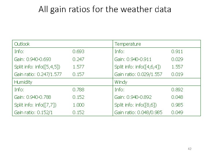
All gain ratios for the weather data Outlook Temperature Info: 0. 693 Info: 0. 911 Gain: 0. 940 -0. 693 0. 247 Gain: 0. 940 -0. 911 0. 029 Split info: info([5, 4, 5]) 1. 577 Split info: info([4, 6, 4]) 1. 557 Gain ratio: 0. 247/1. 577 0. 157 Gain ratio: 0. 029/1. 557 0. 019 Humidity Windy Info: 0. 788 Info: 0. 892 Gain: 0. 940 -0. 788 0. 152 Gain: 0. 940 -0. 892 0. 048 Split info: info([7, 7]) 1. 000 Split info: info([8, 6]) 0. 985 Gain ratio: 0. 152/1 0. 152 Gain ratio: 0. 048/0. 985 0. 049 42

More on the gain ratio • “Outlook” still comes out top • However: “ID code” has greater gain ratio • Standard fix: ad hoc test to prevent splitting on that type of identifier attribute • Problem with gain ratio: it may overcompensate • May choose an attribute just because its intrinsic information is very low • Standard fix: only consider attributes with greater than average information gain • Both tricks are implemented in the well-known C 4. 5 decision tree learner 43

Discussion • Top-down induction of decision trees: ID 3, algorithm developed by Ross Quinlan • Gain ratio just one modification of this basic algorithm • C 4. 5 tree learner deals with numeric attributes, missing values, noisy data • Similar approach: CART tree learner • Uses Gini index rather than entropy to measure impurity • There are many other attribute selection criteria! (But little difference in accuracy of result) 44

Covering algorithms • Can convert decision tree into a rule set • Straightforward, but rule set overly complex • More effective conversions are not trivial and may incur a lot of computation • Instead, we can generate rule set directly • One approach: for each class in turn, find rule set that covers all instances in it (excluding instances not in the class) • Called a covering approach: • At each stage of the algorithm, a rule is identified that “covers” some of the instances 45

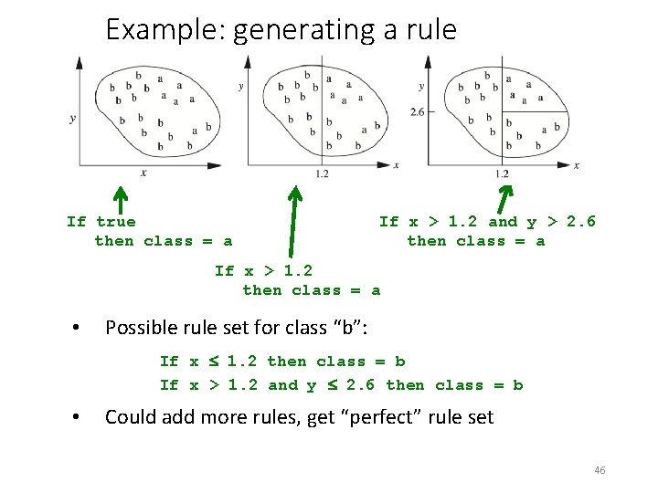
Example: generating a rule If true then class = a If x > 1. 2 and y > 2. 6 then class = a If x > 1. 2 then class = a • Possible rule set for class “b”: If x 1. 2 then class = b If x > 1. 2 and y 2. 6 then class = b • Could add more rules, get “perfect” rule set 46

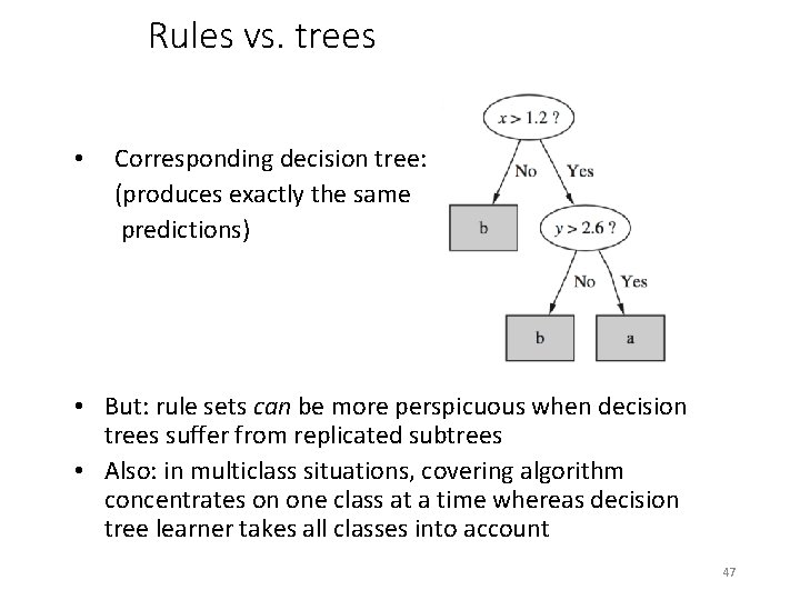
Rules vs. trees • Corresponding decision tree: (produces exactly the same predictions) • But: rule sets can be more perspicuous when decision trees suffer from replicated subtrees • Also: in multiclass situations, covering algorithm concentrates on one class at a time whereas decision tree learner takes all classes into account 47

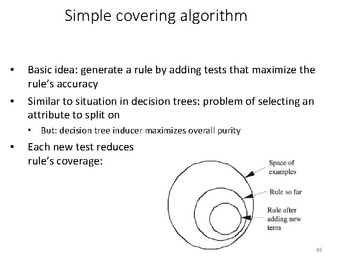
Simple covering algorithm • • Basic idea: generate a rule by adding tests that maximize the rule’s accuracy Similar to situation in decision trees: problem of selecting an attribute to split on • But: decision tree inducer maximizes overall purity • Each new test reduces rule’s coverage: 48

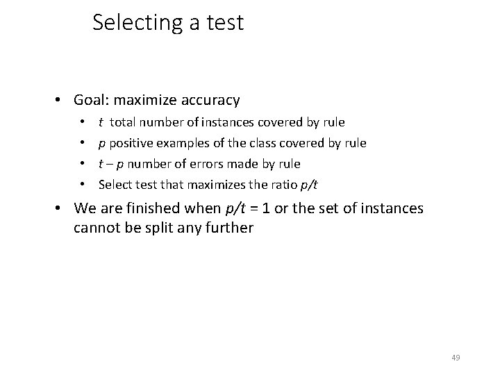
Selecting a test • Goal: maximize accuracy • • t total number of instances covered by rule p positive examples of the class covered by rule t – p number of errors made by rule Select test that maximizes the ratio p/t • We are finished when p/t = 1 or the set of instances cannot be split any further 49

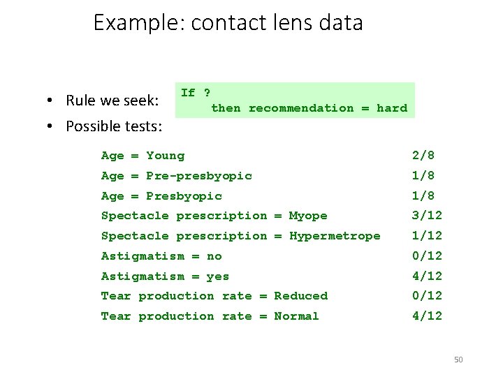
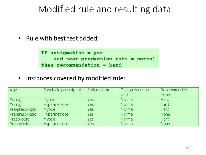
Example: contact lens data • Rule we seek: If ? • Possible tests: then recommendation = hard Age = Young 2/8 Age = Pre-presbyopic 1/8 Age = Presbyopic 1/8 Spectacle prescription = Myope 3/12 Spectacle prescription = Hypermetrope 1/12 Astigmatism = no 0/12 Astigmatism = yes 4/12 Tear production rate = Reduced 0/12 Tear production rate = Normal 4/12 50

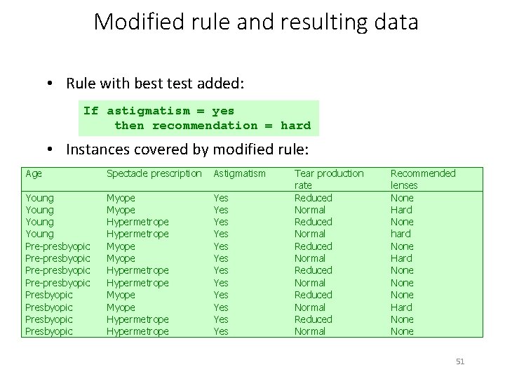
Modified rule and resulting data • Rule with best test added: If astigmatism = yes then recommendation = hard • Instances covered by modified rule: Age Spectacle prescription Astigmatism Young Pre-presbyopic Presbyopic Myope Hypermetrope Myope Hypermetrope Yes Yes Yes Tear production rate Reduced Normal Reduced Normal Recommended lenses None Hard None hard None Hard None 51

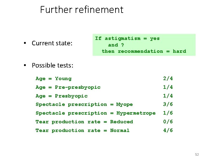
Further refinement • Current state: If astigmatism = yes and ? then recommendation = hard • Possible tests: Age = Young 2/4 Age = Pre-presbyopic 1/4 Age = Presbyopic 1/4 Spectacle prescription = Myope 3/6 Spectacle prescription = Hypermetrope 1/6 Tear production rate = Reduced 0/6 Tear production rate = Normal 4/6 52

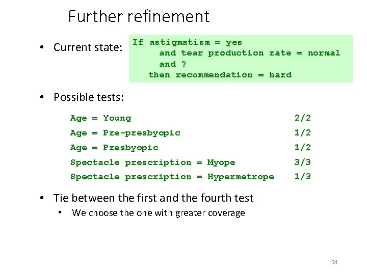
Modified rule and resulting data • Rule with best test added: If astigmatism = yes and tear production rate = normal then recommendation = hard • Instances covered by modified rule: Age Spectacle prescription Astigmatism Young Pre-presbyopic Presbyopic Myope Hypermetrope Yes Yes Yes Tear production rate Normal Normal Recommended lenses Hard hard Hard None 53

Further refinement • Current state: If astigmatism = yes and tear production rate = normal and ? then recommendation = hard • Possible tests: Age = Young 2/2 Age = Pre-presbyopic 1/2 Age = Presbyopic 1/2 Spectacle prescription = Myope 3/3 Spectacle prescription = Hypermetrope 1/3 • Tie between the first and the fourth test • We choose the one with greater coverage 54

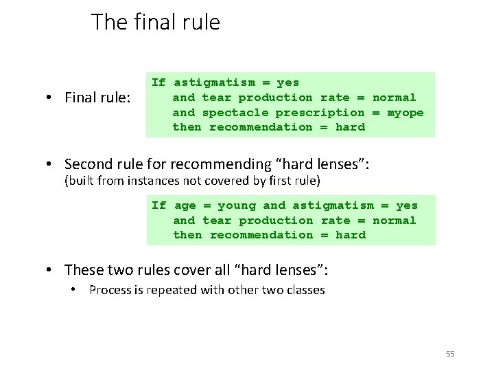
The final rule • Final rule: If astigmatism = yes and tear production rate = normal and spectacle prescription = myope then recommendation = hard • Second rule for recommending “hard lenses”: (built from instances not covered by first rule) If age = young and astigmatism = yes and tear production rate = normal then recommendation = hard • These two rules cover all “hard lenses”: • Process is repeated with other two classes 55

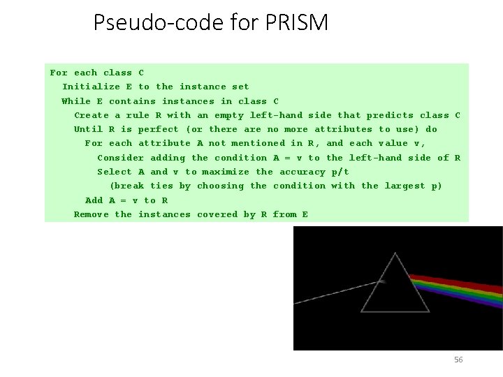
Pseudo-code for PRISM For each class C Initialize E to the instance set While E contains instances in class C Create a rule R with an empty left-hand side that predicts class C Until R is perfect (or there are no more attributes to use) do For each attribute A not mentioned in R, and each value v, Consider adding the condition A = v to the left-hand side of R Select A and v to maximize the accuracy p/t (break ties by choosing the condition with the largest p) Add A = v to R Remove the instances covered by R from E 56

Rules vs. decision lists • PRISM with outer loop removed generates a decision list for one class • Subsequent rules are designed for rules that are not covered by previous rules • But: order does not matter because all rules predict the same class so outcome does not change if rules are shuffled • Outer loop considers all classes separately • No order dependence implied • Problems: overlapping rules, default rule required 57

Separate and conquer rule learning • Rule learning methods like the one PRISM employs (for each class) are called separate-and-conquer algorithms: • First, identify a useful rule • Then, separate out all the instances it covers • Finally, “conquer” the remaining instances • Difference to divide-and-conquer methods: • Subset covered by a rule does not need to be explored any further 58

Mining association rules • Naïve method for finding association rules: • Use separate-and-conquer method • Treat every possible combination of attribute values as a separate class • Two problems: • Computational complexity • Resulting number of rules (which would have to be pruned on the basis of support and confidence) • It turns out that we can look for association rules with high support and accuracy directly 59

Item sets: the basis for finding rules • Support: number of instances correctly covered by association rule • The same as the number of instances covered by all tests in the rule (LHS and RHS!) • Item: one test/attribute-value pair • Item set : all items occurring in a rule • Goal: find only rules that exceed pre-defined support • � Do it by finding all item sets with the given minimum support and generating rules from them! 60

Weather data Outlook Temp Humidity Windy Play Sunny Hot High False No Sunny Hot High True No Overcast Hot High False Yes Rainy Mild High False Yes Rainy Cool Normal True No Overcast Cool Normal True Yes Sunny Mild High False No Sunny Cool Normal False Yes Rainy Mild Normal False Yes Sunny Mild Normal True Yes Overcast Mild High True Yes Overcast Hot Normal False Yes Rainy Mild High True No 61

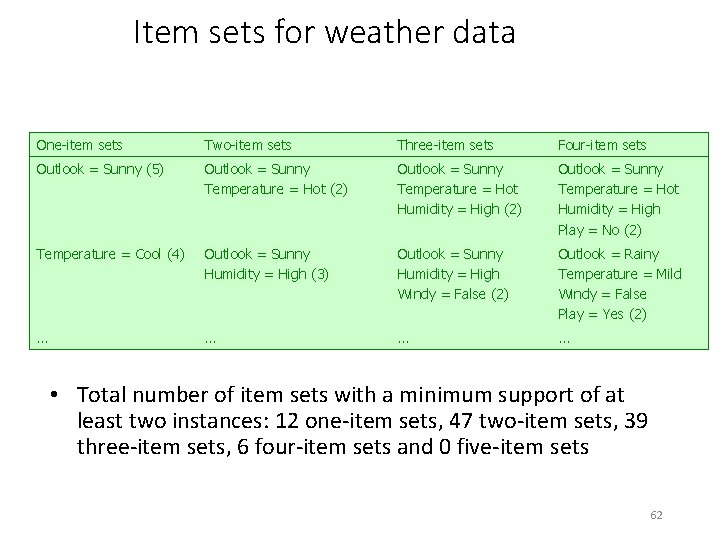
Item sets for weather data One-item sets Two-item sets Three-item sets Four-item sets Outlook = Sunny (5) Outlook = Sunny Temperature = Hot (2) Outlook = Sunny Temperature = Hot Humidity = High Play = No (2) Temperature = Cool (4) Outlook = Sunny Humidity = High (3) Outlook = Sunny Humidity = High Windy = False (2) Outlook = Rainy Temperature = Mild Windy = False Play = Yes (2) … … • Total number of item sets with a minimum support of at least two instances: 12 one-item sets, 47 two-item sets, 39 three-item sets, 6 four-item sets and 0 five-item sets 62

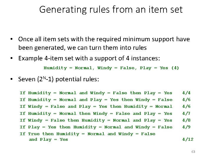
Generating rules from an item set • Once all item sets with the required minimum support have been generated, we can turn them into rules • Example 4 -item set with a support of 4 instances: Humidity = Normal, Windy = False, Play = Yes (4) • Seven (2 N-1) potential rules: If If Humidity = Normal and Windy = False then Play = Yes Humidity = Normal and Play = Yes then Windy = False and Play = Yes then Humidity = Normal then Windy = False and Play = Yes Windy = False then Humidity = Normal and Play = Yes then Humidity = Normal and Windy = False True then Humidity = Normal and Windy = False and Play = Yes 4/4 4/6 4/7 4/8 4/9 4/12 63

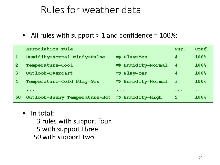
Rules for weather data • All rules with support > 1 and confidence = 100%: Association rule Sup. Conf. 1 Humidity=Normal Windy=False Play=Yes 4 100% 2 Temperature=Cool Humidity=Normal 4 100% 3 Outlook=Overcast Play=Yes 4 100% 4 Temperature=Cold Play=Yes Humidity=Normal 3 100% . . . 2 100% 58 Outlook=Sunny Temperature=Hot Humidity=High • In total: 3 rules with support four 5 with support three 50 with support two 64

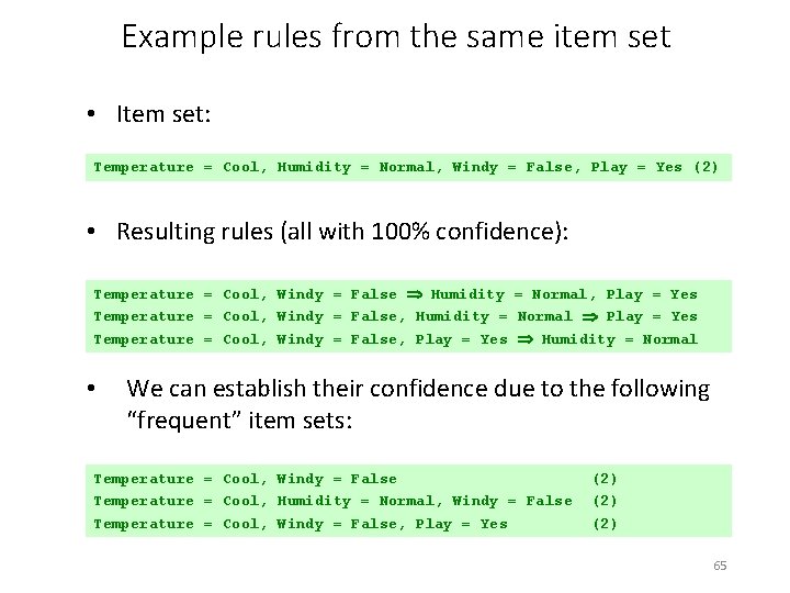
Example rules from the same item set • Item set: Temperature = Cool, Humidity = Normal, Windy = False, Play = Yes (2) • Resulting rules (all with 100% confidence): Temperature = Cool, Windy = False Humidity = Normal, Play = Yes Temperature = Cool, Windy = False, Humidity = Normal Play = Yes Temperature = Cool, Windy = False, Play = Yes Humidity = Normal • We can establish their confidence due to the following “frequent” item sets: Temperature = Cool, Windy = False Temperature = Cool, Humidity = Normal, Windy = False Temperature = Cool, Windy = False, Play = Yes (2) (2) 65

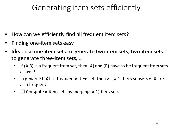
Generating item sets efficiently • How can we efficiently find all frequent item sets? • Finding one-item sets easy • Idea: use one-item sets to generate two-item sets, two-item sets to generate three-item sets, … • If (A B) is a frequent item set, then (A) and (B) have to be frequent item sets as well! • In general: if X is a frequent k-item set, then all (k-1)-item subsets of X are also frequent • � Compute k-item sets by merging (k-1)-item sets 66

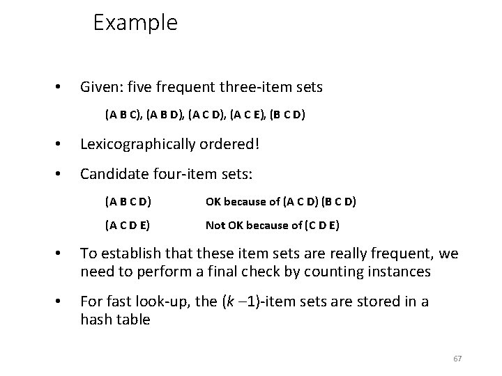
Example • Given: five frequent three-item sets (A B C), (A B D), (A C E), (B C D) • Lexicographically ordered! • Candidate four-item sets: (A B C D) OK because of (A C D) (B C D) (A C D E) Not OK because of (C D E) • To establish that these item sets are really frequent, we need to perform a final check by counting instances • For fast look-up, the (k – 1)-item sets are stored in a hash table 67

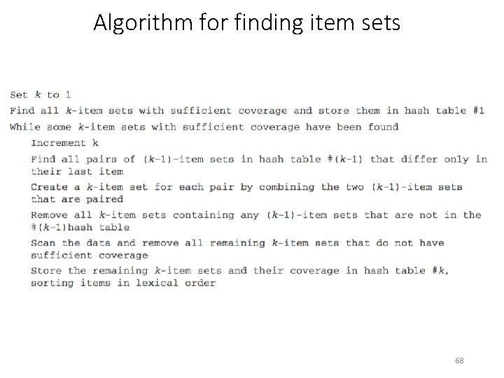
Algorithm for finding item sets 68

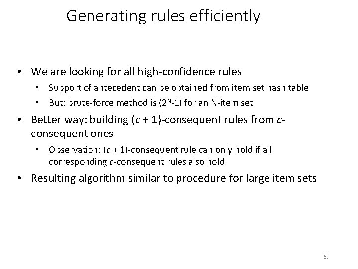
Generating rules efficiently • We are looking for all high-confidence rules • Support of antecedent can be obtained from item set hash table • But: brute-force method is (2 N-1) for an N-item set • Better way: building (c + 1)-consequent rules from cconsequent ones • Observation: (c + 1)-consequent rule can only hold if all corresponding c-consequent rules also hold • Resulting algorithm similar to procedure for large item sets 69

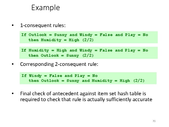
Example • 1 -consequent rules: If Outlook = Sunny and Windy = False and Play = No then Humidity = High (2/2) If Humidity = High and Windy = False and Play = No then Outlook = Sunny (2/2) • Corresponding 2 -consequent rule: If Windy = False and Play = No then Outlook = Sunny and Humidity = High (2/2) • Final check of antecedent against item set hash table is required to check that rule is actually sufficiently accurate 70

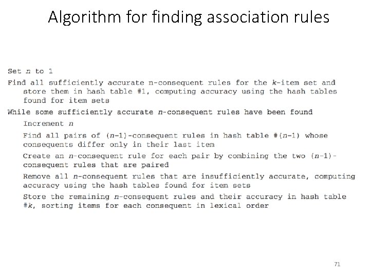
Algorithm for finding association rules 71

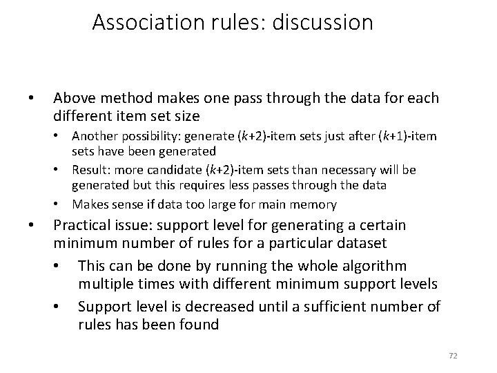
Association rules: discussion • Above method makes one pass through the data for each different item set size • Another possibility: generate (k+2)-item sets just after (k+1)-item sets have been generated • Result: more candidate (k+2)-item sets than necessary will be generated but this requires less passes through the data • Makes sense if data too large for main memory • Practical issue: support level for generating a certain minimum number of rules for a particular dataset • This can be done by running the whole algorithm multiple times with different minimum support levels • Support level is decreased until a sufficient number of rules has been found 72

Other issues • Standard ARFF format very inefficient for typical market basket data • Attributes represent items in a basket and most items are usually missing from any particular basket • Data should be represented in sparse format • Note on terminology: instances are also called transactions in the literature on association rule mining • Confidence is not necessarily the best measure • Example: milk occurs in almost every supermarket transaction • Other measures have been devised (e. g. , lift) • It is often quite difficult to find interesting patterns in the large number of association rules that can be generated 73

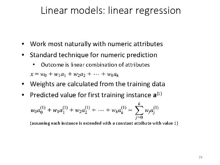
Linear models: linear regression • Work most naturally with numeric attributes • Standard technique for numeric prediction • Outcome is linear combination of attributes • Weights are calculated from the training data • Predicted value for first training instance a(1) (assuming each instance is extended with a constant attribute with value 1) 74

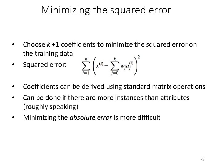
Minimizing the squared error • • • Choose k +1 coefficients to minimize the squared error on the training data Squared error: Coefficients can be derived using standard matrix operations Can be done if there are more instances than attributes (roughly speaking) Minimizing the absolute error is more difficult 75

Classification • Any regression technique can be used for classification • Training: perform a regression for each class, setting the output to 1 for training instances that belong to class, and 0 for those that don’t • Prediction: predict class corresponding to model with largest output value (membership value) • For linear regression this method is also known as multiresponse linear regression • Problem: membership values are not in the [0, 1] range, so they cannot be considered proper probability estimates • In practice, they are often simply clipped into the [0, 1] range and normalized to sum to 1 76

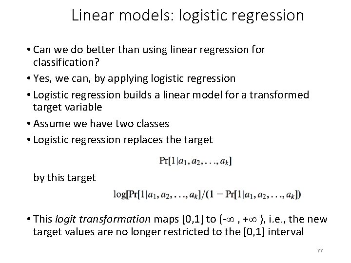
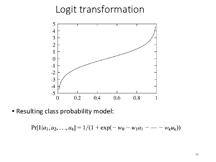
Linear models: logistic regression • Can we do better than using linear regression for classification? • Yes, we can, by applying logistic regression • Logistic regression builds a linear model for a transformed target variable • Assume we have two classes • Logistic regression replaces the target by this target • This logit transformation maps [0, 1] to (-¥ , +¥ ), i. e. , the new target values are no longer restricted to the [0, 1] interval 77

Logit transformation • Resulting class probability model: 78

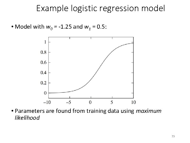
Example logistic regression model • Model with w 0 = -1. 25 and w 1 = 0. 5: • Parameters are found from training data using maximum likelihood 79

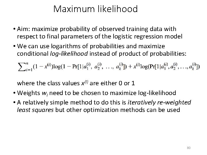
Maximum likelihood • Aim: maximize probability of observed training data with respect to final parameters of the logistic regression model • We can use logarithms of probabilities and maximize conditional log-likelihood instead of product of probabilities: where the class values x(i) are either 0 or 1 • Weights wi need to be chosen to maximize log-likelihood • A relatively simple method to do this is iteratively re-weighted least squares but other optimization methods can be used 80

Multiple classes • Logistic regression for two classes is also called binomial logistic regression • What do we do when have a problem with k classes? • Can perform logistic regression independently for each class (like in multi-response linear regression) • Problem: the probability estimates for the different classes will generally not sum to one • Better: train k-1 coupled linear models by maximizing likelihood over all classes simultaneously • This is known as multi-class logistic regression, multinomial logistic regression or polytomous logistic regression • Alternative multi-class approach that often works well in practice: pairwise classification 81

Pairwise classification • Idea: build model for each pair of classes, using only training data from those classes • Classifications are derived by voting: given a test instance, let each model vote for one of its two classes • Problem? Have to train k(k-1)/2 two-classification models for a k-class problem • Turns out not to be a problem in many cases because pairwise training sets become small: • Assume data evenly distributed, i. e. , 2 n/k instances per learning problem for n instances in total • Suppose training time of learning algorithm is linear in n • Then runtime for the training process is proportional to (k(k-1)/2)×(2 n/k) = (k-1)n, i. e. , linear in the number of classes and the number of instances • Even more beneficial if learning algorithm scales worse than linearly 82

Linear models are hyperplanes • Decision boundary for two-class logistic regression is where probability equals 0. 5: which occurs when • Thus logistic regression can only separate data that can be separated by a hyperplane • Multi-response linear regression has the same problem. Class 1 is assigned if: 83

Linear models: the perceptron • Observation: we do not actually need probability estimates if all we want to do is classification • Different approach: learn separating hyperplane directly • Let us assume the data is linearly separable • In that case there is a simple algorithm for learning a separating hyperplane called the perceptron learning rule • Hyperplane: where we again assume that there is a constant attribute with value 1 (bias) • If the weighted sum is greater than zero we predict the first class, otherwise the second class 84

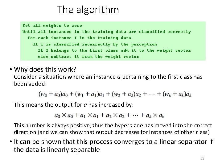
The algorithm Set all weights to zero Until all instances in the training data are classified correctly For each instance I in the training data If I is classified incorrectly by the perceptron If I belongs to the first class add it to the weight vector else subtract it from the weight vector • Why does this work? Consider a situation where an instance a pertaining to the first class has been added: This means the output for a has increased by: This number is always positive, thus the hyperplane has moved into the correct direction (and we can show that output decreases for instances of other class) • It can be shown that this process converges to a linear separator if the data is linearly separable 85

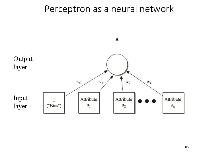
Perceptron as a neural network Output layer Input layer 86

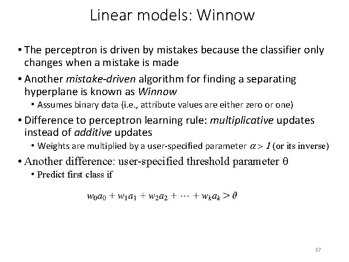
Linear models: Winnow • The perceptron is driven by mistakes because the classifier only changes when a mistake is made • Another mistake-driven algorithm for finding a separating hyperplane is known as Winnow • Assumes binary data (i. e. , attribute values are either zero or one) • Difference to perceptron learning rule: multiplicative updates instead of additive updates • Weights are multiplied by a user-specified parameter a > 1 (or its inverse) • Another difference: user-specified threshold parameter q • Predict first class if 87

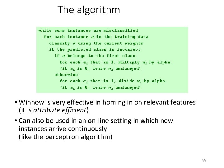
The algorithm while some instances are misclassified for each instance a in the training data classify a using the current weights if the predicted class is incorrect if a belongs to the first class for each ai that is 1, multiply wi by alpha (if ai is 0, leave wi unchanged) otherwise for each ai that is 1, divide wi by alpha (if ai is 0, leave wi unchanged) • Winnow is very effective in homing in on relevant features (it is attribute efficient) • Can also be used in an on-line setting in which new instances arrive continuously (like the perceptron algorithm) 88

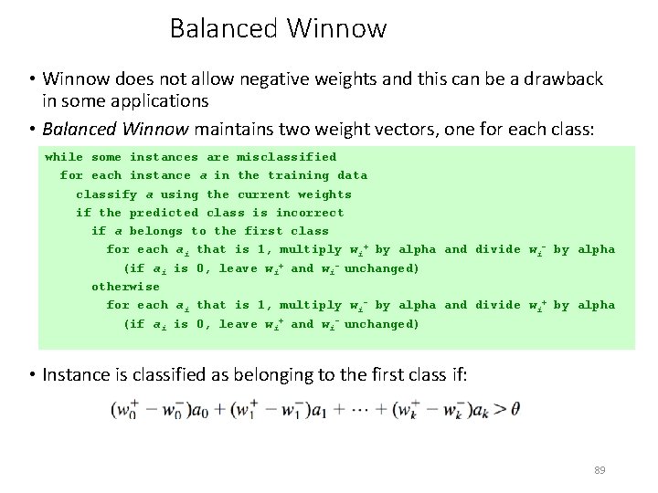
Balanced Winnow • Winnow does not allow negative weights and this can be a drawback in some applications • Balanced Winnow maintains two weight vectors, one for each class: while some instances are misclassified for each instance a in the training data classify a using the current weights if the predicted class is incorrect if a belongs to the first class for each ai that is 1, multiply wi+ by alpha and divide wi- by alpha (if ai is 0, leave wi+ and wi- unchanged) otherwise for each ai that is 1, multiply wi- by alpha and divide wi+ by alpha (if ai is 0, leave wi+ and wi- unchanged) • Instance is classified as belonging to the first class if: 89

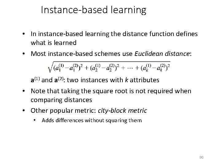
Instance-based learning • In instance-based learning the distance function defines what is learned • Most instance-based schemes use Euclidean distance: a(1) and a(2): two instances with k attributes • Note that taking the square root is not required when comparing distances • Other popular metric: city-block metric • Adds differences without squaring them 90

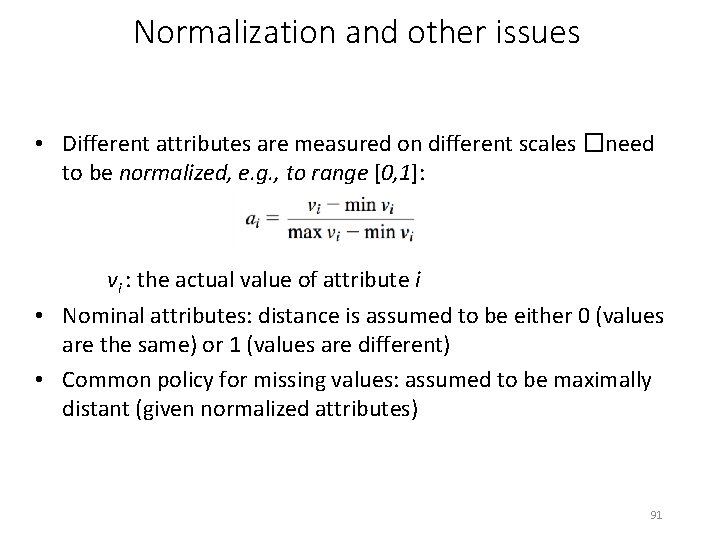
Normalization and other issues • Different attributes are measured on different scales �need to be normalized, e. g. , to range [0, 1]: vi : the actual value of attribute i • Nominal attributes: distance is assumed to be either 0 (values are the same) or 1 (values are different) • Common policy for missing values: assumed to be maximally distant (given normalized attributes) 91

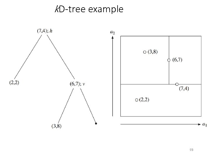
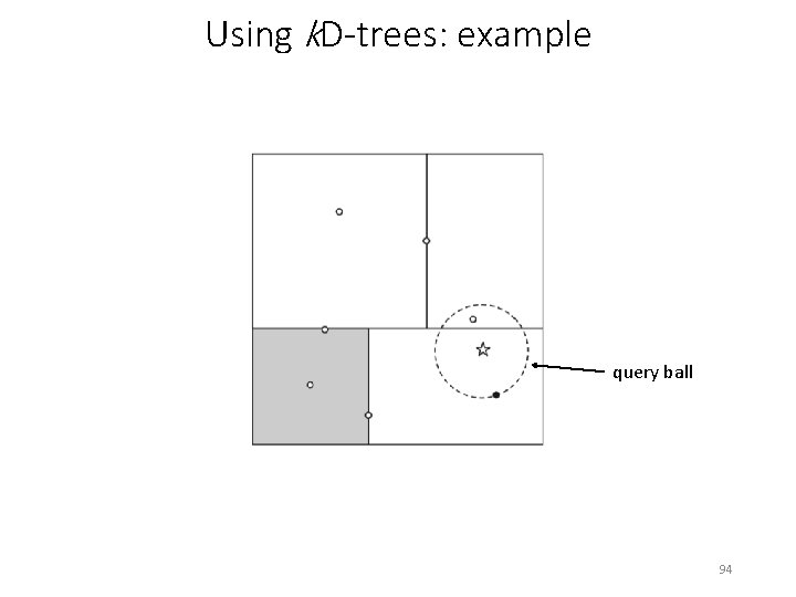
Finding nearest neighbors efficiently • Simplest way of finding nearest neighbour: linear scan of the data • Classification takes time proportional to the product of the number of instances in training and test sets • Nearest-neighbor search can be done more efficiently using appropriate data structures • We will discuss two methods that represent training data in a tree structure: k. D-trees and ball trees 92

k. D-tree example 93

Using k. D-trees: example query ball 94

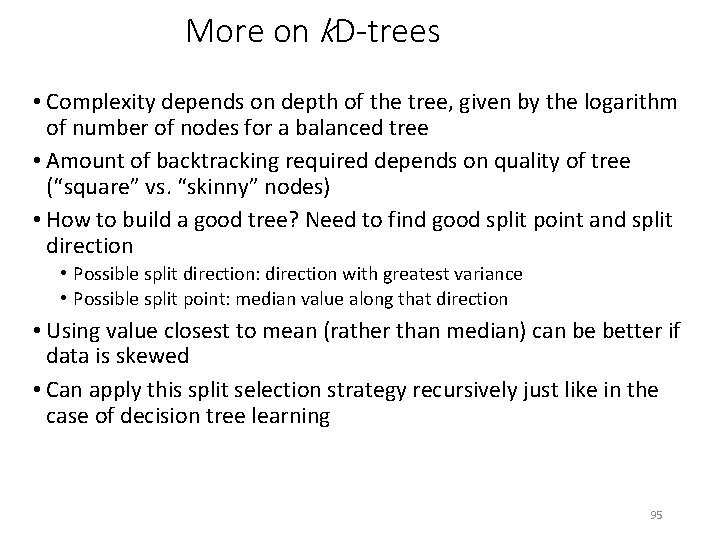
More on k. D-trees • Complexity depends on depth of the tree, given by the logarithm of number of nodes for a balanced tree • Amount of backtracking required depends on quality of tree (“square” vs. “skinny” nodes) • How to build a good tree? Need to find good split point and split direction • Possible split direction: direction with greatest variance • Possible split point: median value along that direction • Using value closest to mean (rather than median) can be better if data is skewed • Can apply this split selection strategy recursively just like in the case of decision tree learning 95

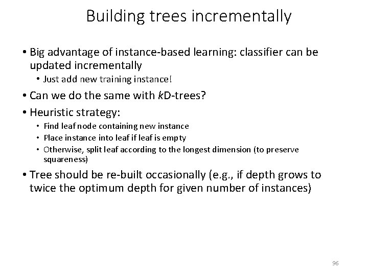
Building trees incrementally • Big advantage of instance-based learning: classifier can be updated incrementally • Just add new training instance! • Can we do the same with k. D-trees? • Heuristic strategy: • Find leaf node containing new instance • Place instance into leaf if leaf is empty • Otherwise, split leaf according to the longest dimension (to preserve squareness) • Tree should be re-built occasionally (e. g. , if depth grows to twice the optimum depth for given number of instances) 96

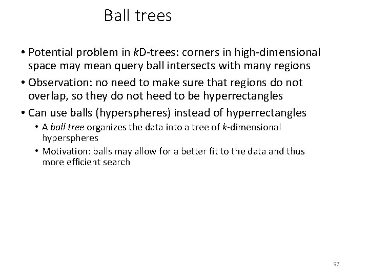
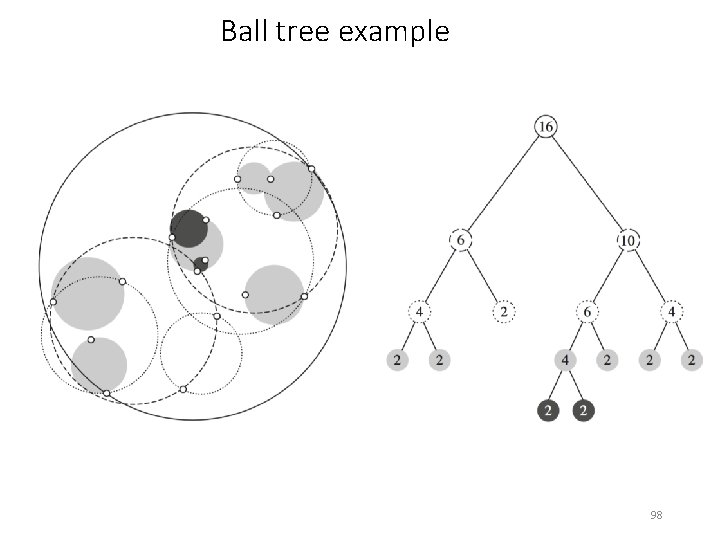
Ball trees • Potential problem in k. D-trees: corners in high-dimensional space may mean query ball intersects with many regions • Observation: no need to make sure that regions do not overlap, so they do not heed to be hyperrectangles • Can use balls (hyperspheres) instead of hyperrectangles • A ball tree organizes the data into a tree of k-dimensional hyperspheres • Motivation: balls may allow for a better fit to the data and thus more efficient search 97

Ball tree example 98

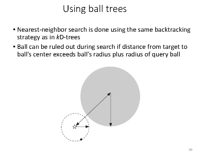
Using ball trees • Nearest-neighbor search is done using the same backtracking strategy as in k. D-trees • Ball can be ruled out during search if distance from target to ball's center exceeds ball's radius plus radius of query ball 99

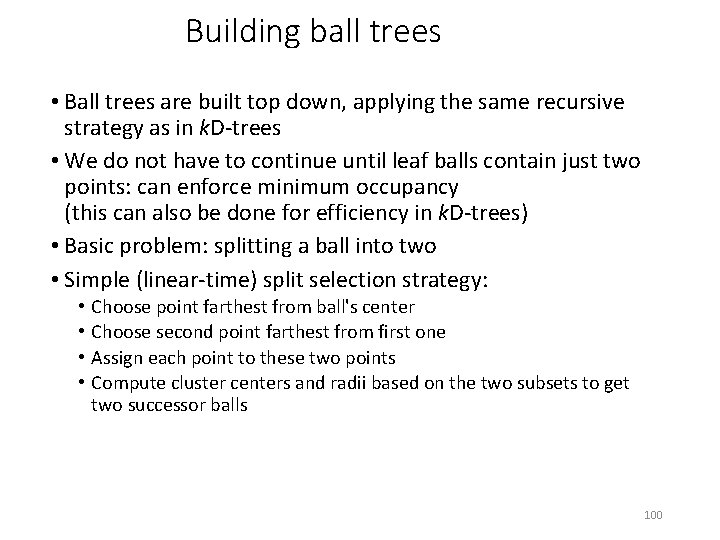
Building ball trees • Ball trees are built top down, applying the same recursive strategy as in k. D-trees • We do not have to continue until leaf balls contain just two points: can enforce minimum occupancy (this can also be done for efficiency in k. D-trees) • Basic problem: splitting a ball into two • Simple (linear-time) split selection strategy: • • Choose point farthest from ball's center Choose second point farthest from first one Assign each point to these two points Compute cluster centers and radii based on the two subsets to get two successor balls 100

Discussion of nearest-neighbor learning • Often very accurate • Assumes all attributes are equally important • Remedy: attribute selection, attribute weights, or attribute scaling • Possible remedies against noisy instances: • Take a majority vote over the k nearest neighbors • Remove noisy instances from dataset (difficult!) • Statisticians have used k-NN since the early 1950 s • If n ��and k/n � 0, classification error approaches minimum • k. D-trees can become inefficient when the number of attributes is too large • Ball trees are instances may help; they are instances of metric trees 101

Clustering • Clustering techniques apply when there is no class to be predicted: they perform unsupervised learning • Aim: divide instances into “natural” groups • As we have seen, clusters can be: • disjoint vs. overlapping • deterministic vs. probabilistic • flat vs. hierarchical • We will look at a classic clustering algorithm called k-means • k-means clusters are disjoint, deterministic, and flat 102

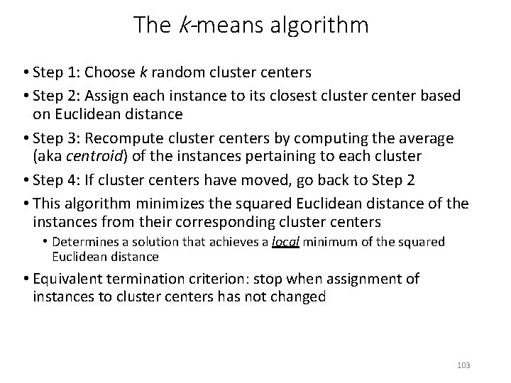
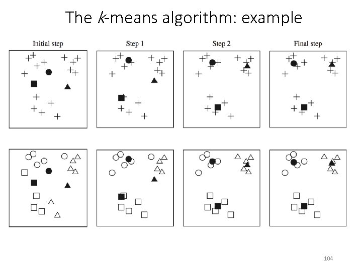
The k-means algorithm • Step 1: Choose k random cluster centers • Step 2: Assign each instance to its closest cluster center based on Euclidean distance • Step 3: Recompute cluster centers by computing the average (aka centroid) of the instances pertaining to each cluster • Step 4: If cluster centers have moved, go back to Step 2 • This algorithm minimizes the squared Euclidean distance of the instances from their corresponding cluster centers • Determines a solution that achieves a local minimum of the squared Euclidean distance • Equivalent termination criterion: stop when assignment of instances to cluster centers has not changed 103

The k-means algorithm: example 104

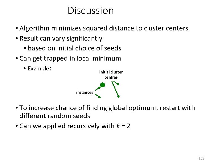
Discussion • Algorithm minimizes squared distance to cluster centers • Result can vary significantly • based on initial choice of seeds • Can get trapped in local minimum • Example: initial cluster centres instances • To increase chance of finding global optimum: restart with different random seeds • Can we applied recursively with k = 2 105

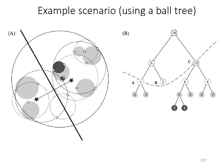
Faster distance calculations • Can we use k. D-trees or ball trees to speed up the process? Yes, we can: • First, build the tree data structure, which remains static, for all the data points • At each node, store the number of instances and the sum of all instances (summary statistics) • In each iteration of k-means, descend the tree and find out which cluster each node belongs to • Can stop descending as soon as we find out that a node belongs entirely to a particular cluster • Use summary statistics stored previously at the nodes to compute new cluster centers 106

Example scenario (using a ball tree) 107

Choosing the number of clusters • Big question in practice: what is the right number of clusters, i. e. , what is the right value for k? • Cannot simply optimize squared distance on training data to choose k • Squared distance decreases monotonically with increasing values of k • Need some measure that balances distance with complexity of the model, e. g. , based on the MDL principle (covered later) • Finding the right-size model using MDL becomes easier when applying a recursive version of k-means (bisecting k-means): • Compute A: information required to store data centroid, and the location of each instance with respect to this centroid • Split data into two clusters using 2 -means • Compute B: information required to store the two new cluster centroids, and the location of each instance with respect to these two • If A > B, split the data and recurse (just like in other tree learners) 108

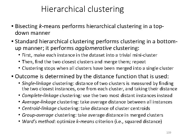
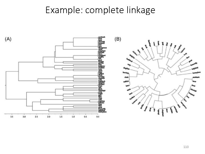
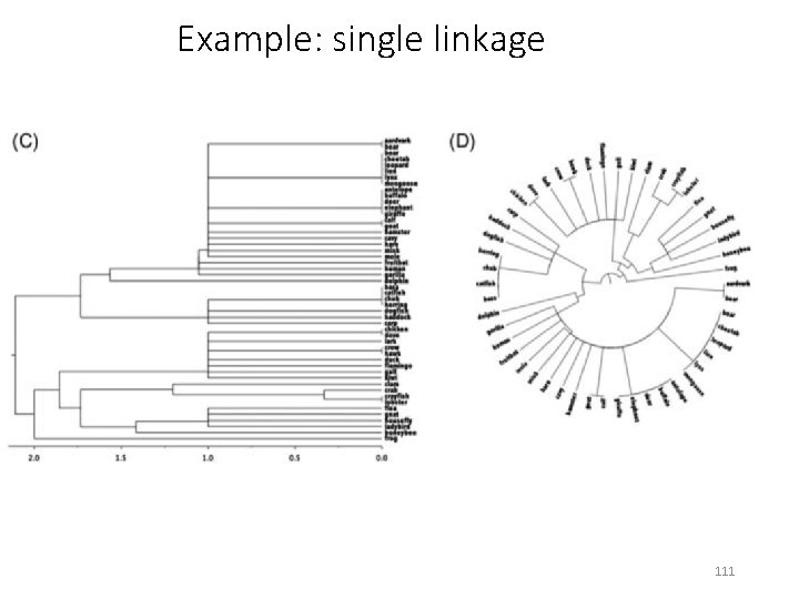
Hierarchical clustering • Bisecting k-means performs hierarchical clustering in a topdown manner • Standard hierarchical clustering performs clustering in a bottomup manner; it performs agglomerative clustering: • First, make each instance in the dataset into a trivial mini-cluster • Then, find the two closest clusters and merge them; repeat • Clustering stops when all clusters have been merged into a single cluster • Outcome is determined by the distance function that is used: • Single-linkage clustering: distance of two clusters is measured by finding the two closest instances, one from each cluster, and taking their distance • Complete-linkage clustering: use the two most distant instances instead • Average-linkage clustering: take average distance between all instances • Centroid-linkage clustering: take distance of cluster centroids • Group-average clustering: take average distance in merged clusters • Ward’s method: optimize k-means criterion (i. e. , squared distance) 109

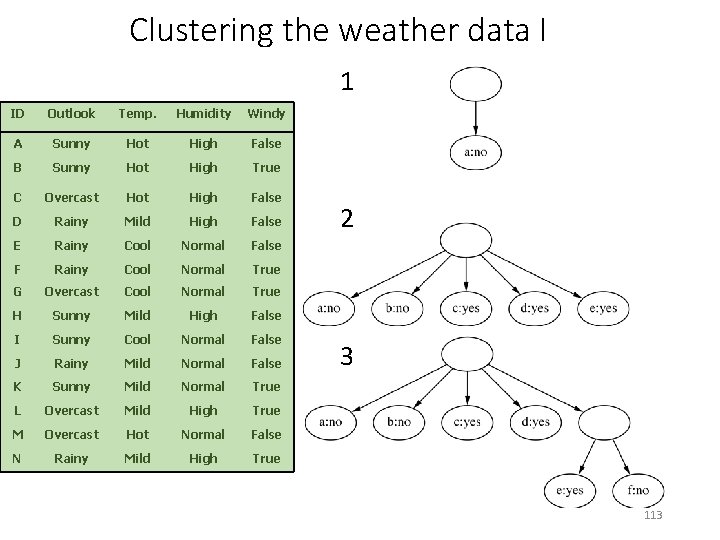
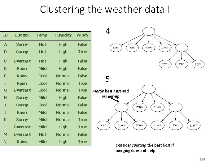
Example: complete linkage 110

Example: single linkage 111

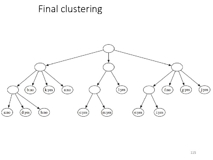
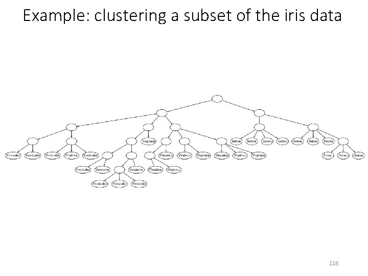
Incremental clustering • Heuristic approach (COBWEB/CLASSIT) • Forms a hierarchy of clusters incrementally • Start: • tree consists of empty root node • Then: • add instances one by one • update tree appropriately at each stage • to update, find the right leaf for an instance • may involve restructuring the tree using merging or splitting of nodes • Update decisions are based on a goodness measure called category utility 112

Clustering the weather data I 1 ID Outlook Temp. Humidity Windy A Sunny Hot High False B Sunny Hot High True C Overcast Hot High False D Rainy Mild High False E Rainy Cool Normal False F Rainy Cool Normal True G Overcast Cool Normal True H Sunny Mild High False I Sunny Cool Normal False J Rainy Mild Normal False K Sunny Mild Normal True L Overcast Mild High True M Overcast Hot Normal False N Rainy Mild High True 2 3 113

Clustering the weather data II ID Outlook Temp. Humidity Windy A Sunny Hot High False B Sunny Hot High True C Overcast Hot High False D Rainy Mild High False E Rainy Cool Normal False F Rainy Cool Normal True G Overcast Cool Normal True H Sunny Mild High False I Sunny Cool Normal False J Rainy Mild Normal False K Sunny Mild Normal True L Overcast Mild High True M Overcast Hot Normal False N Rainy Mild High True 4 5 Merge best host and runner-up 3 Consider splitting the best host if merging does not help 114

Final clustering 115

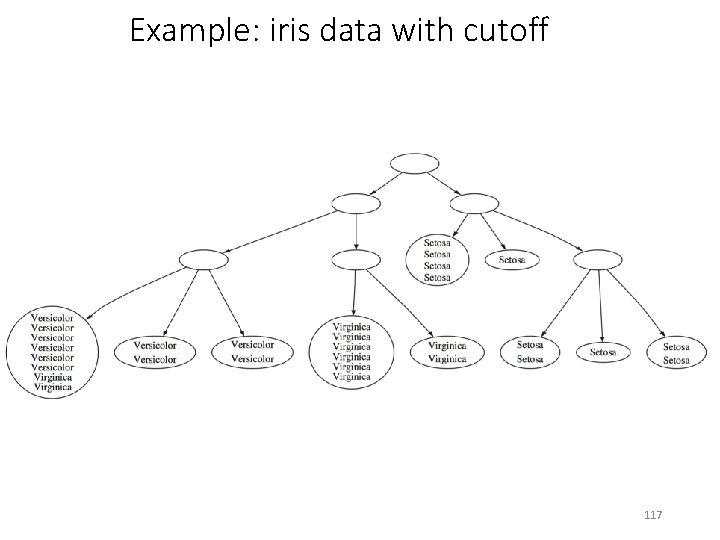
Example: clustering a subset of the iris data 116

Example: iris data with cutoff 117

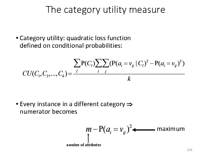
The category utility measure • Category utility: quadratic loss function defined on conditional probabilities: • Every instance in a different category numerator becomes maximum number of attributes 118

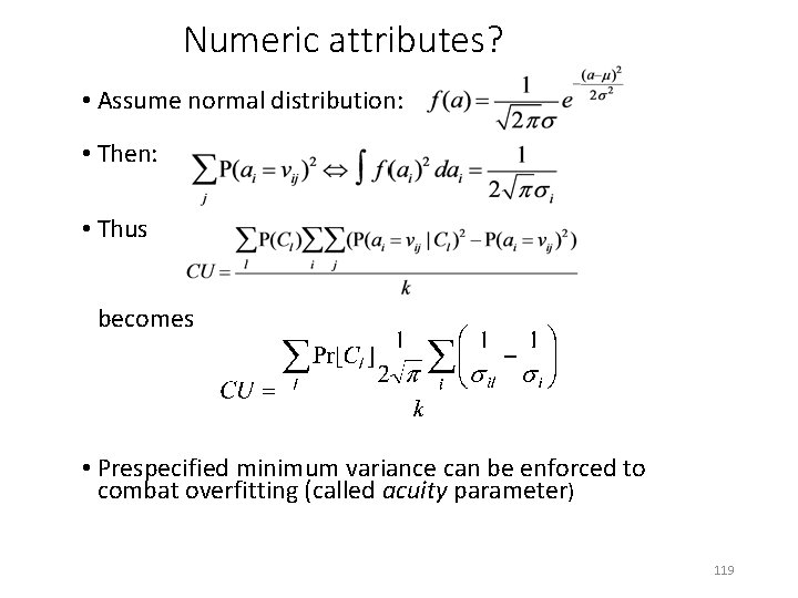
Numeric attributes? • Assume normal distribution: • Then: • Thus becomes • Prespecified minimum variance can be enforced to combat overfitting (called acuity parameter) 119

Multi-instance learning • Recap: multi-instance learning is concerned with examples corresponding to sets (really, bags or multi-sets) of instances • All instances have the same attributes but the full set of instances is split into subsets of related instances that are not necessarily independent • These subsets are the examples for learning • Example applications of multi-instance learning: image classification, classification of molecules • Simplicity-first methodology can be applied to multi-instance learning with surprisingly good results • Two simple approaches to multi-instance learning, both using standard single-instance learners: • Manipulate the input to learning • Manipulate the output of learning 120

Aggregating the input • Idea: convert multi-instance learning problem into a singleinstance one • Summarize the instances in a bag by computing the mean, mode, minimum and maximum, etc. , of each attribute as new attributes • “Summary” instance retains the class label of its bag • To classify a new bag the same process is used • Any single-instance learning method, e. g. , decision tree learning, can be applied to the resulting data • This approach discards most of the information in a bag of instances but works surprisingly well in practice • Should be used as a base line when evaluating more advanced approaches to multi-instance learning • More sophisticated region-based summary statistics can be applied to extend this basic approach 121

Aggregating the output • Idea: learn a single-instance classifier directly from the original instances in all the bags • Each instance is given the class of the bag it originates from • But: bags can contain differing numbers of instances give each instance a weight inversely proportional to the bag's size • To classify a new bag: • Produce a prediction for each instance in the bag • Aggregate the predictions to produce a prediction for the bag as a whole • One approach: treat predictions as votes for the various class labels; alternatively, average the class probability estimates • This approach treats all instances as independent at training time, which is not the case in true multi-instance applications • Nevertheless, it often works very well in practice and should be used as a base line 122

Some final comments on the basic methods • Bayes’ rule stems from his “Essay towards solving a problem in the doctrine of chances” (1763) • Difficult bit in general: estimating prior probabilities (easy in the case of naïve Bayes) • Extension of naïve Bayes: Bayesian networks (which we will discuss later) • The algorithm for association rules we discussed is called APRIORI; many other algorithms exist • Minsky and Papert (1969) showed that linear classifiers have limitations, e. g. , can’t learn a logical XOR of two attributes • But: combinations of them can (this yields multi-layer neural nets, which we will discuss later) 123