Data Mining Practical Machine Learning Tools and Techniques

Data Mining Practical Machine Learning Tools and Techniques Slides for Chapter 6, Trees and Rules of Data Mining by I. H. Witten, E. Frank, M. A. Hall and C. J. Pal

Algorithms for learning trees and rules • Decision trees • From ID 3 to C 4. 5 (pruning, numeric attributes, . . . ) • Classification rules • From PRISM to RIPPER and PART (pruning, numeric data, …) • Association Rules • Faster rule mining with frequent-pattern trees 2

Decision Trees 3

Industrial-strength algorithms • For an algorithm to be useful in a wide range of real-world applications it must: • Permit numeric attributes • Allow missing values • Be robust in the presence of noise • Basic scheme needs to be extended to fulfill these requirements 4

From ID 3 to C 4. 5 • Extending ID 3: • to permit numeric attributes: straightforward • to deal sensibly with missing values: trickier • stability for noisy data: requires pruning mechanism • End result: C 4. 5 (Quinlan) • Best-known and (probably) most widely-used learning algorithm • Commercial successor: C 5. 0 5

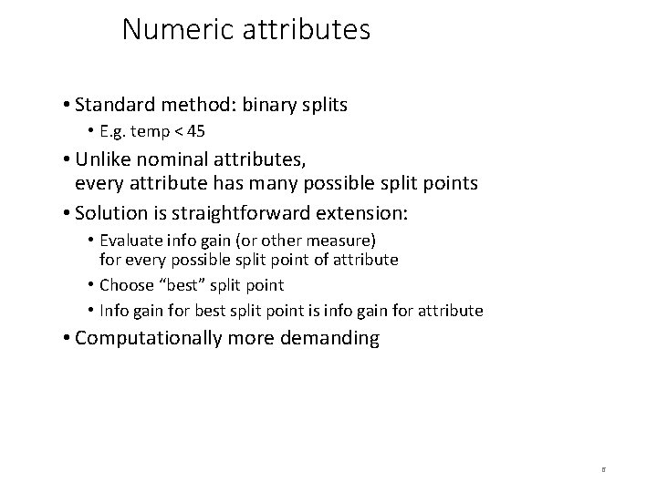
Numeric attributes • Standard method: binary splits • E. g. temp < 45 • Unlike nominal attributes, every attribute has many possible split points • Solution is straightforward extension: • Evaluate info gain (or other measure) for every possible split point of attribute • Choose “best” split point • Info gain for best split point is info gain for attribute • Computationally more demanding 6

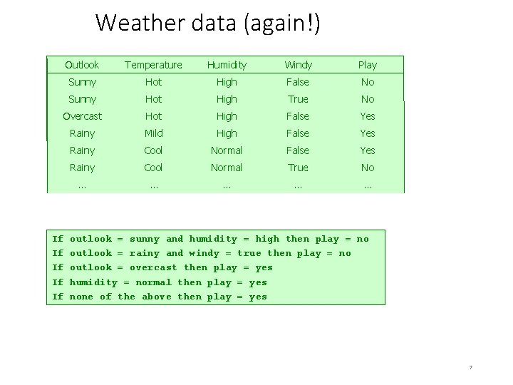
Weather data (again!) Outlook Temperature Humidity Windy Play Sunny Hot High False No Sunny Hot High True No Overcast Hot High False Yes Rainy Mild Normal High False Yes … Rainy … Cool … Normal … False … Yes Rainy … Cool … Normal … True … No … … … If If If outlook = sunny and humidity = high then play = no outlook = rainy and windy = true then play = no outlook = overcast then play = yes humidity = normal then play = yes none of the above then play = yes 7

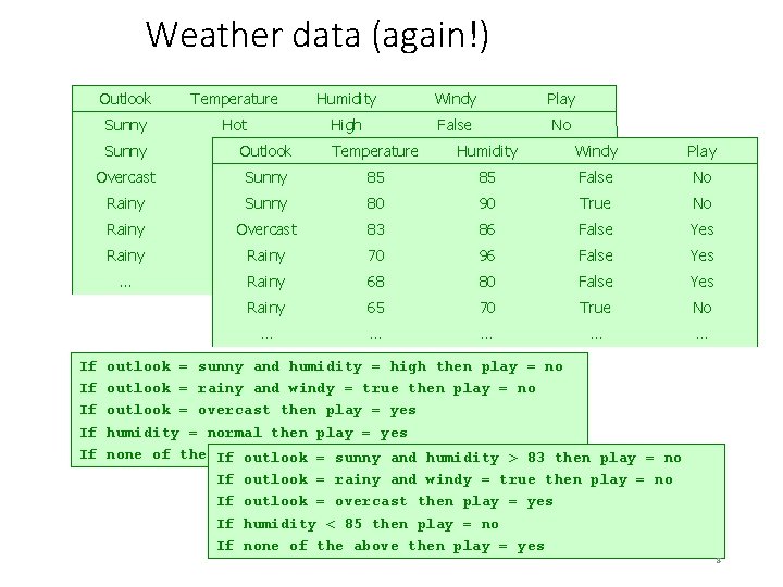
Weather data (again!) Outlook Temperature Humidity Windy Play Sunny Hot High False No Sunny Hot. Outlook High Temperature True Humidity No Windy Play Overcast Hot. Sunny High Hot 85 False. High 85 Yes False No Rainy Mild. Sunny 80 Normal High Hot 90 False. High Yes True No … Rainy …Overcast Cool … Hot 83 Normal … High 86 False … False Yes Rainy … Cool … Rainy Normal … Mild 70 True … Normal 96 No … False Yes … … … Rainy … … 68 … 80 … … False … Yes Rainy … 65 … 70 … True … No … … … If If If … outlook = sunny and humidity = high then play = no outlook = rainy and windy = true then play = no outlook = overcast then play = yes humidity = normal then play = yes none of the If above then = play = yes outlook sunny and humidity > 83 then play = no If outlook = rainy and windy = true then play = no If outlook = overcast then play = yes If humidity < 85 then play = no If none of the above then play = yes 8

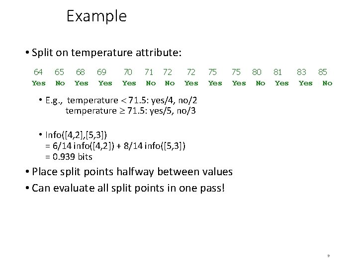
Example • Split on temperature attribute: 64 Yes 65 No 68 Yes 69 Yes 70 Yes 71 72 No No 72 Yes 75 80 Yes No 81 Yes 83 85 Yes No • E. g. , temperature 71. 5: yes/4, no/2 temperature 71. 5: yes/5, no/3 • Info([4, 2], [5, 3]) = 6/14 info([4, 2]) + 8/14 info([5, 3]) = 0. 939 bits • Place split points halfway between values • Can evaluate all split points in one pass! 9

Can avoid repeated sorting • Sort instances by the values of the numeric attribute • Time complexity for sorting: O (n log n) • Does this have to be repeated at each node of the tree? • No! Sort order for children can be derived from sort order for parent • Time complexity of derivation: O (n) • Drawback: need to create and store an array of sorted indices for each numeric attribute 10

Binary vs multiway splits • Splitting (multi-way) on a nominal attribute exhausts all information in that attribute • Nominal attribute is tested (at most) once on any path in the tree • Not so for binary splits on numeric attributes! • Numeric attribute may be tested several times along a path in the tree • Disadvantage: tree is hard to read • Remedy: • pre-discretize numeric attributes, or • use multi-way splits instead of binary ones 11

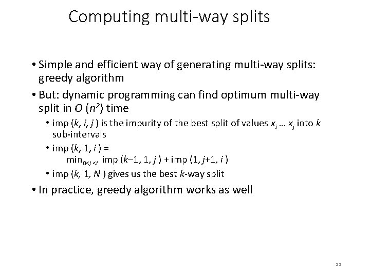
Computing multi-way splits • Simple and efficient way of generating multi-way splits: greedy algorithm • But: dynamic programming can find optimum multi-way split in O (n 2) time • imp (k, i, j ) is the impurity of the best split of values xi … xj into k sub-intervals • imp (k, 1, i ) = min 0<j <i imp (k– 1, 1, j ) + imp (1, j+1, i ) • imp (k, 1, N ) gives us the best k-way split • In practice, greedy algorithm works as well 12

Missing values • C 4. 5 applies method of fractional instances: • Split instances with missing values into pieces • A piece going down a branch receives a weight proportional to the popularity of the branch • weights sum to 1 • Info gain works with fractional instances • use sums of weights instead of counts • During classification, split the instance into pieces in the same way • Merge probability distribution using weights 13

Pruning • Prevent overfitting the training data: “prune the decision tree • Two strategies: • Postpruning take a fully-grown decision tree and discard unreliable parts • Prepruning stop growing a branch when information becomes unreliable • Postpruning is preferred in practice—prepruning can “stop early” 14

Prepruning • Based on statistical significance test • Stop growing the tree when there is no statistically significant association between any attribute and the class at a particular node • Most popular test: chi-squared test • Quinlan’s classic tree learner ID 3 used chi-squared test in addition to information gain • Only statistically significant attributes were allowed to be selected by the information gain procedure 15

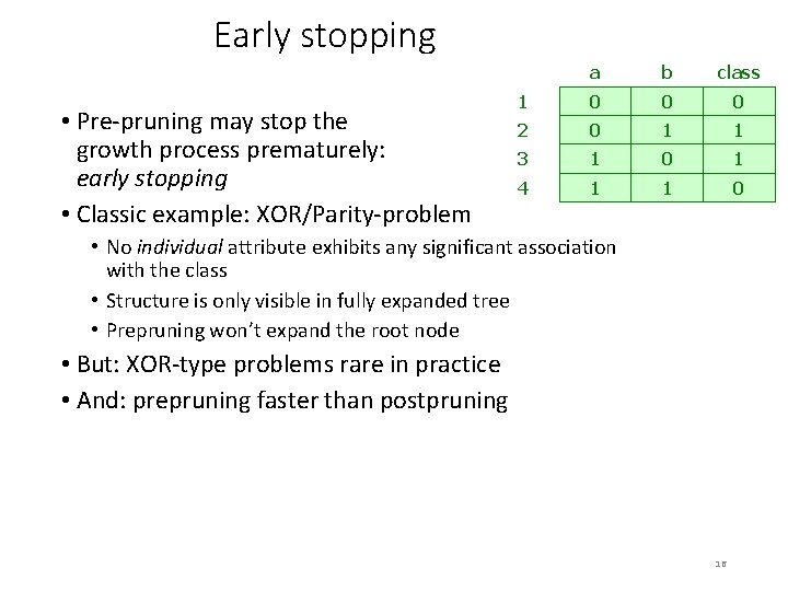
Early stopping • Pre-pruning may stop the growth process prematurely: early stopping • Classic example: XOR/Parity-problem a b class 1 0 0 0 2 0 1 1 3 1 0 1 4 1 1 0 • No individual attribute exhibits any significant association with the class • Structure is only visible in fully expanded tree • Prepruning won’t expand the root node • But: XOR-type problems rare in practice • And: prepruning faster than postpruning 16

Postpruning • First, build full tree • Then, prune it • Fully-grown tree shows all attribute interactions • Problem: some subtrees might be due to chance effects • Two pruning operations: • Subtree replacement • Subtree raising • Possible strategies: • error estimation • significance testing • MDL principle 17

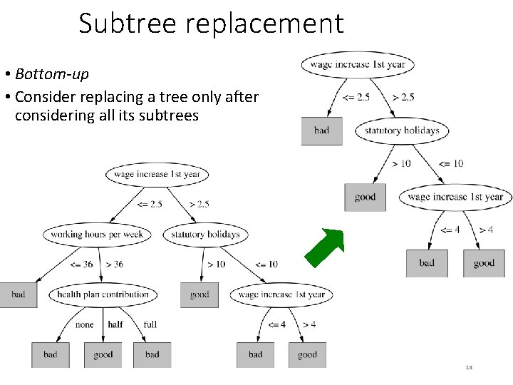
Subtree replacement • Bottom-up • Consider replacing a tree only after considering all its subtrees 18

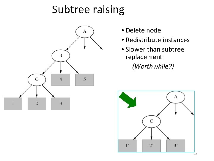
Subtree raising • Delete node • Redistribute instances • Slower than subtree replacement (Worthwhile? ) 19

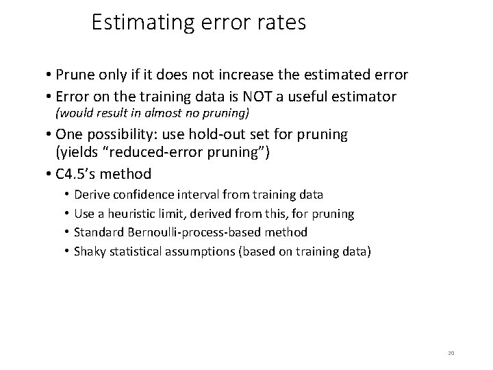
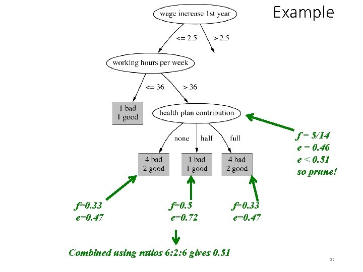
Estimating error rates • Prune only if it does not increase the estimated error • Error on the training data is NOT a useful estimator (would result in almost no pruning) • One possibility: use hold-out set for pruning (yields “reduced-error pruning”) • C 4. 5’s method • • Derive confidence interval from training data Use a heuristic limit, derived from this, for pruning Standard Bernoulli-process-based method Shaky statistical assumptions (based on training data) 20

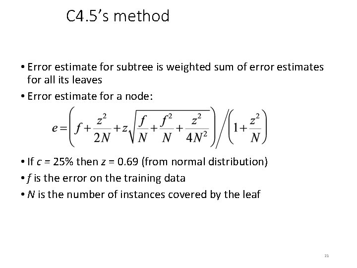
C 4. 5’s method • Error estimate for subtree is weighted sum of error estimates for all its leaves • Error estimate for a node: • If c = 25% then z = 0. 69 (from normal distribution) • f is the error on the training data • N is the number of instances covered by the leaf 21

Example f = 5/14 e = 0. 46 e < 0. 51 so prune! f=0. 33 e=0. 47 f=0. 5 e=0. 72 Combined using ratios 6: 2: 6 gives 0. 51 f=0. 33 e=0. 47 22

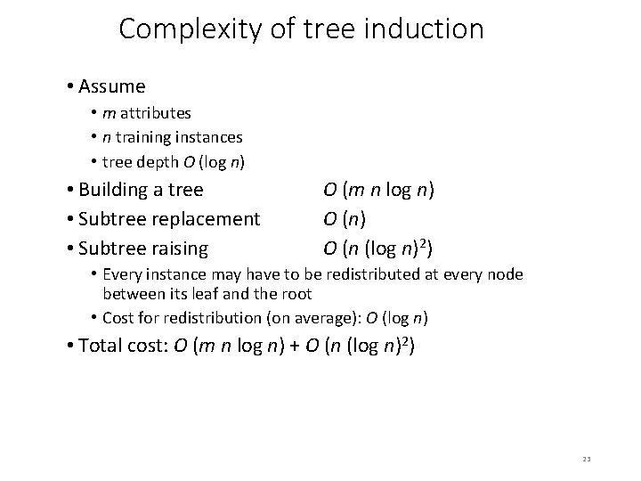
Complexity of tree induction • Assume • m attributes • n training instances • tree depth O (log n) • Building a tree • Subtree replacement • Subtree raising O (m n log n) O (n (log n)2) • Every instance may have to be redistributed at every node between its leaf and the root • Cost for redistribution (on average): O (log n) • Total cost: O (m n log n) + O (n (log n)2) 23

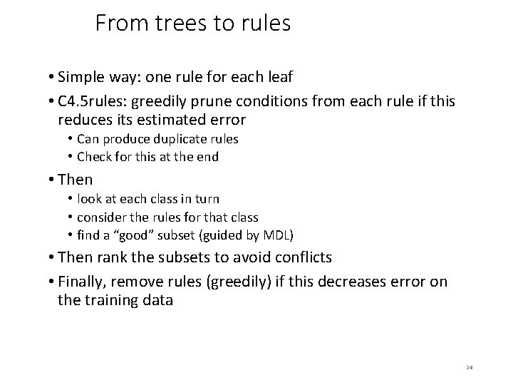
From trees to rules • Simple way: one rule for each leaf • C 4. 5 rules: greedily prune conditions from each rule if this reduces its estimated error • Can produce duplicate rules • Check for this at the end • Then • look at each class in turn • consider the rules for that class • find a “good” subset (guided by MDL) • Then rank the subsets to avoid conflicts • Finally, remove rules (greedily) if this decreases error on the training data 24

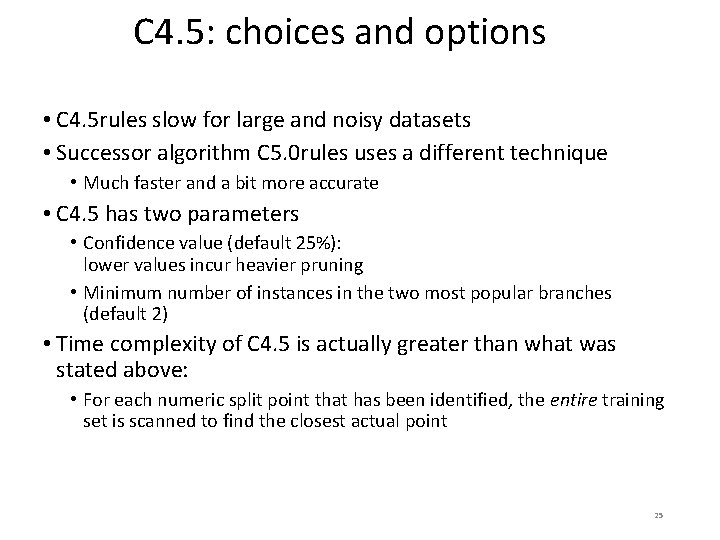
C 4. 5: choices and options • C 4. 5 rules slow for large and noisy datasets • Successor algorithm C 5. 0 rules uses a different technique • Much faster and a bit more accurate • C 4. 5 has two parameters • Confidence value (default 25%): lower values incur heavier pruning • Minimum number of instances in the two most popular branches (default 2) • Time complexity of C 4. 5 is actually greater than what was stated above: • For each numeric split point that has been identified, the entire training set is scanned to find the closest actual point 25

Cost-complexity pruning • C 4. 5's postpruning often does not prune enough • Tree size continues to grow when more instances are added even if performance on independent data does not improve • But: it is very fast and popular in practice • Can be worthwhile in some cases to strive for a more compact tree at the expense of more computational effort • Cost-complexity pruning method from the CART (Classification and Regression Trees) learning system achieves this • Applies cross-validation or a hold-out set to choose an appropriate tree size for the final tree 26

Cost-complexity pruning details • Basic idea: • First prune subtrees that, relative to their size, lead to the smallest increase in error on the training data • Increase in error (α): average error increase per leaf of subtree • Bottom-up pruning based on this criterion generates a sequence of successively smaller trees • Each candidate tree in the sequence corresponds to one particular threshold value αi • Which tree to chose as the final model? • Use either a hold-out set or cross-validation to estimate the error for each αi • Rebuild tree on entire training set using chosen value of α 27

Discussion TDIDT: Top-Down Induction of Decision Trees • The most extensively studied method of machine learning used in data mining • Different criteria for attribute/test selection rarely make a large difference • Different pruning methods mainly change the size of the resulting pruned tree • C 4. 5 builds univariate decision trees: each node tests a single attribute • Some TDITDT systems can build multivariate trees (e. g. , the famous CART tree learner) 28

Discussion and Bibliographic Notes • CART’s pruning method (Breiman et al. 1984) can often produce smaller trees than C 4. 5’s method • C 4. 5’s overfitting problems have been investigated empirically by Oates and Jensen (1997) • A complete description of C 4. 5, the early 1990 s version, appears as a excellent and readable book (Quinlan 1993) • An MDL-based heuristic for C 4. 5 Release 8 that combats overfitting of numeric attributes is described by Quinlan (1998) • The more recent version of Quinlan’s tree learner, C 5. 0, is also available as open-source code 29

Classification Rules 30

Classification rules • Common procedure: separate-and-conquer • Differences: • • • Search method (e. g. greedy, beam search, . . . ) Test selection criteria (e. g. accuracy, . . . ) Pruning method (e. g. MDL, hold-out set, . . . ) Stopping criterion (e. g. minimum accuracy) Post-processing step • Also: Decision list vs. one rule set for each class 31

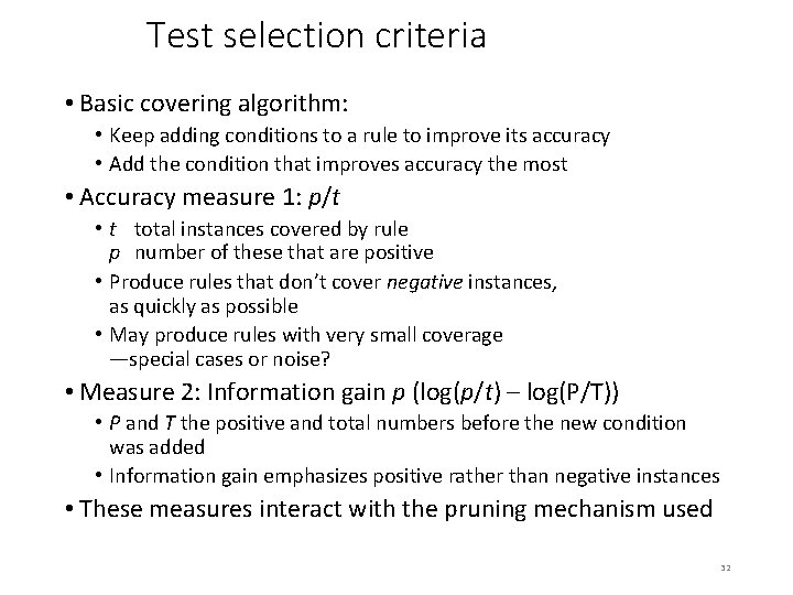
Test selection criteria • Basic covering algorithm: • Keep adding conditions to a rule to improve its accuracy • Add the condition that improves accuracy the most • Accuracy measure 1: p/t • t total instances covered by rule p number of these that are positive • Produce rules that don’t cover negative instances, as quickly as possible • May produce rules with very small coverage —special cases or noise? • Measure 2: Information gain p (log(p/t) – log(P/T)) • P and T the positive and total numbers before the new condition was added • Information gain emphasizes positive rather than negative instances • These measures interact with the pruning mechanism used 32

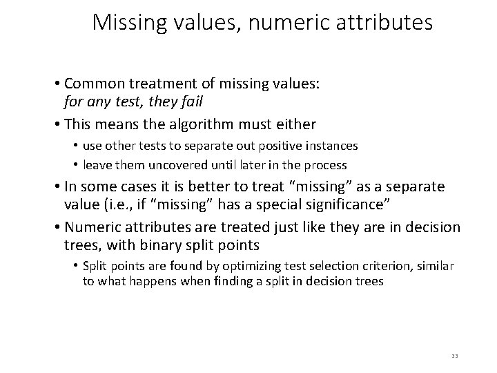
Missing values, numeric attributes • Common treatment of missing values: for any test, they fail • This means the algorithm must either • use other tests to separate out positive instances • leave them uncovered until later in the process • In some cases it is better to treat “missing” as a separate value (i. e. , if “missing” has a special significance” • Numeric attributes are treated just like they are in decision trees, with binary split points • Split points are found by optimizing test selection criterion, similar to what happens when finding a split in decision trees 33

Pruning rules • Two main strategies: • Incremental pruning • Global pruning • Other difference: pruning criterion • Error on hold-out set (reduced-error pruning) • Statistical significance • MDL principle • Also: post-pruning vs. pre-pruning 34

Using a pruning set • For statistical validity, must evaluate measure on data not used for growing the tree: • This requires a growing set and a pruning set • The full training set is split, randomly, into these two sets • Reduced-error pruning : build full rule set on growing set and then prune it • Incremental reduced-error pruning : simplify each rule as soon as it has been built • Can re-split data after rule has been pruned • Stratification is advantageous when applying reduced-error pruning, so that class proportions are preserved 35

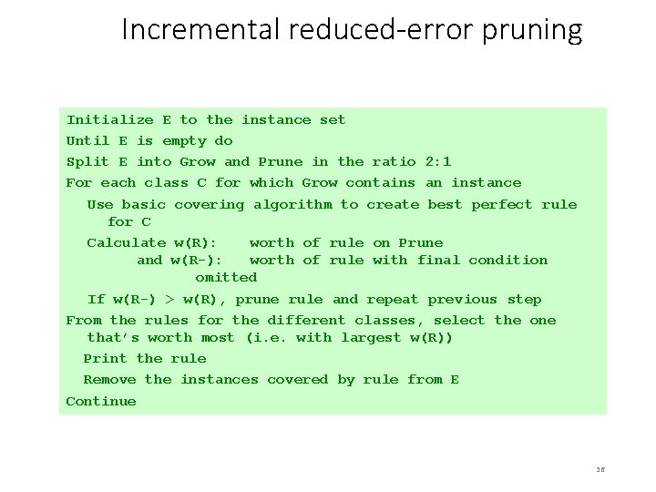
Incremental reduced-error pruning Initialize E to the instance set Until E is empty do Split E into Grow and Prune in the ratio 2: 1 For each class C for which Grow contains an instance Use basic covering algorithm to create best perfect rule for C Calculate w(R): worth of rule on Prune and w(R-): worth of rule with final condition omitted If w(R-) > w(R), prune rule and repeat previous step From the rules for the different classes, select the one that’s worth most (i. e. with largest w(R)) Print the rule Remove the instances covered by rule from E Continue 36

Measures of worth used in IREP • [p + (N – n)] / T • (N is total number of negatives) • Counterintuitive: • p = 2000 and n = 1000 vs. p = 1000 and n = 1 • Success rate p / t • Problem: p = 1 and t = 1 vs. p = 1000 and t = 1001 • (p – n) / t • Same effect as success rate because it equals 2 p/t – 1 • Seems hard to find a simple measure of a rule’s worth that corresponds with intuition 37

Variations • Generating rules for classes in order, from smallest class to largest class • Start with the smallest class and learn a rule set for this class, treating all other classes together as the negative class • Remove the smallest class and proceed to learn a rule set for the next-largest class, and so on • Leave the largest class to be covered by the default rule • Stopping criterion • Stop rule production for each if accuracy becomes too low • Rule learner RIPPER applies this strategy • Employs an MDL-based stopping criterion • Employs a post-processing step to modify the generated rules, guided by a criterion based on the MDL principle 38

Rule learning using global optimization • RIPPER: Repeated Incremental Pruning to Produce Error Reduction • Performs global optimization in an efficient way • Classes are processed in order of increasing size • Initial rule set for each class is generated using IREP • An MDL-based stopping condition is used • DL: bits needs to send examples wrt set of rules, bits needed to send k tests, and bits for k • Once a rule set has been produced for each class, each rule is re -considered and two variants are produced • One is an extended version, one is grown from scratch • Chooses among three candidates according to DL • Final cleanup step greedily deletes rules to minimize DL 39

PART: rule learning using partial trees • PART rule learner avoids global optimization step used in C 4. 5 rules and RIPPER • Generates an unrestricted decision list using the basic separate-and-conquer procedure • In each iteration of the separate-and-conquer algorithm, a rule predicting any of the classes may be added to the rule set • Builds a partial decision tree to obtain each rule • Once partial tree has been generated, one of the leaves of this tree is turned into a rule • A rule is only pruned if all its implications are known • Prevents hasty generalization • Uses C 4. 5’s tree building procedures to build a tree 40

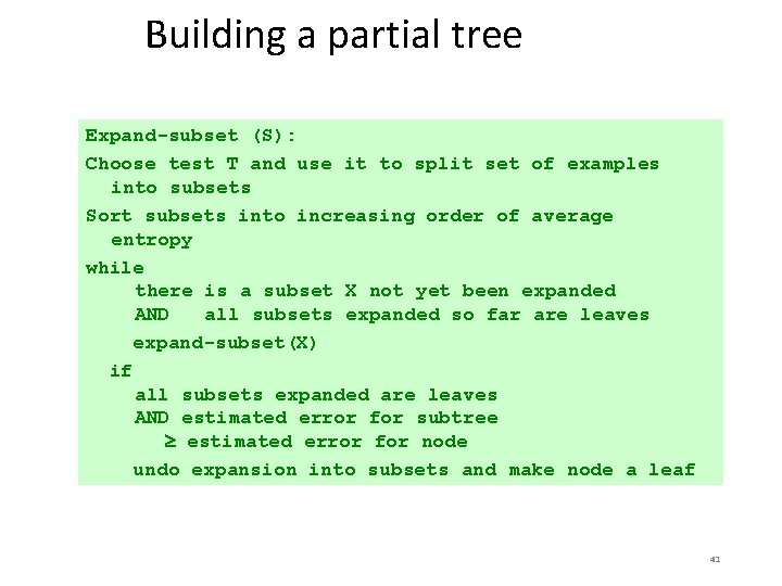
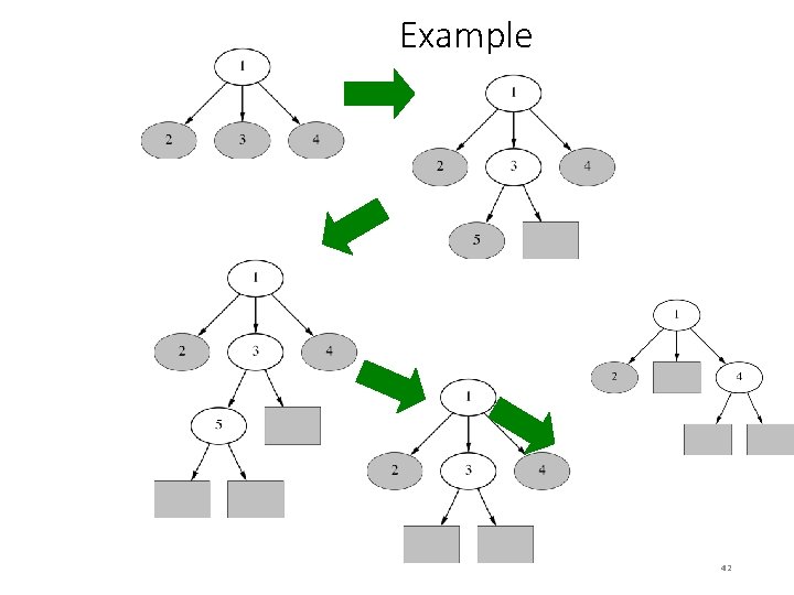
Building a partial tree Expand-subset (S): Choose test T and use it to split set of examples into subsets Sort subsets into increasing order of average entropy while there is a subset X not yet been expanded AND all subsets expanded so far are leaves expand-subset(X) if all subsets expanded are leaves AND estimated error for subtree estimated error for node undo expansion into subsets and make node a leaf 41

Example 42

Notes on PART • Make leaf with maximum coverage into a rule • Treat missing values just as C 4. 5 does i. e. split instance with a missing value into pieces • Time taken to generate a rule: • Worst case: same as for building a pruned C 4. 5 tree - Occurs when data is noisy and the maximum amount of pruning occurs • Best case: same as for building a single if-then rule using the basic strategy employed by the PRISM rule learner - Occurs when data is noise free and no pruning occurs 43

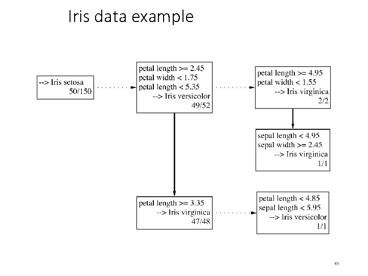
Rules with exceptions • Assume we have a way of generating a single good rule • Then, in principle, it is easy to generate rules with exceptions • Algorithm for building a tree of rules: 1. 2. 3. Select default class for top-level rule Generate a good rule for one of the remaining classes Apply this method recursively to the two subsets produced by the rule (i. e. , instances that are covered/not covered) 44

Iris data example Exceptions are represented as Dotted paths, alternatives as solid ones. 45

Discussion and Bibliographic Notes • The idea of incremental reduced-error pruning is due to Fürnkranz and Widmer (1994) • The RIPPER rule learner is due to Cohen (1995) • What we have presented here is the basic idea of the algorithm; there are many more details in the implementation • An extensive theoretical study of various test selection criteria for rules has been performed by Fürnkranz and Flach (2005) • The rule-learning scheme based on partial decision trees was developed by Frank and Witten (1998) • The procedure for generating rules with exceptions was part of Gaines and Compton’s Induct system (1995) • They called rules with exceptions ripple-down rules • Richards and Compton (1998) describe their role as an alternative to classic knowledge engineering 46

Association Rules 47

Association rules • The Apriori algorithm finds frequent item sets via a generate-and-test methodology • Successively longer item sets are formed from shorter ones • Each different size of candidate item set requires a full scan of the dataset • Combinatorial nature of generation process is costly – particularly if there are many item sets, or item sets are large • Appropriate data structures can help • The FP-growth algorithm for finding frequent item sets employs an extended prefix tree (FP-tree) 48

FP-growth • FP-growth uses a Frequent Pattern Tree (FP-tree) to store a compressed version of the data • Only two passes through a dataset are required to map the data into an FP-tree • The tree is then processed recursively to “grow” large item sets directly • Avoids generating and testing candidate item sets against the entire database 49

Building a frequent pattern tree 1) First pass over the data: count the number times individual items occur 2) Second pass over the data: before inserting each instance into the FP-tree, sort its items in descending order of their frequency of occurrence - Individual items that do not meet the minimum support are not inserted into the tree - Ideally, many instances will share items that occur frequently individually, resulting in a high degree of compression close to the root of the tree 50

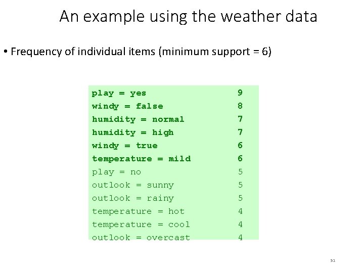
An example using the weather data • Frequency of individual items (minimum support = 6) play = yes windy = false humidity = normal humidity = high windy = true temperature = mild play = no outlook = sunny outlook = rainy temperature = hot temperature = cool outlook = overcast 9 8 7 7 6 6 5 5 5 4 4 4 51

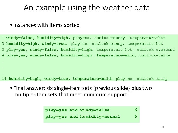
An example using the weather data • Instances with items sorted 1 windy=false, humidity=high, play=no, outlook=sunny, temperature=hot 2 humidity=high, windy=true, play=no, outlook=sunny, temperature=hot 3 play=yes, windy=false, humidity=high, temperature=hot, outlook=overcast 4 play=yes, windy=false, humidity=high, temperature=mild, outlook=rainy. . . 14 humidity=high, windy=true, temperature=mild, play=no, outlook=rainy • Final answer: six single-item sets (previous slide) plus two multiple-item sets that meet minimum support play=yes and windy=false play=yes and humidity=normal 6 6 52

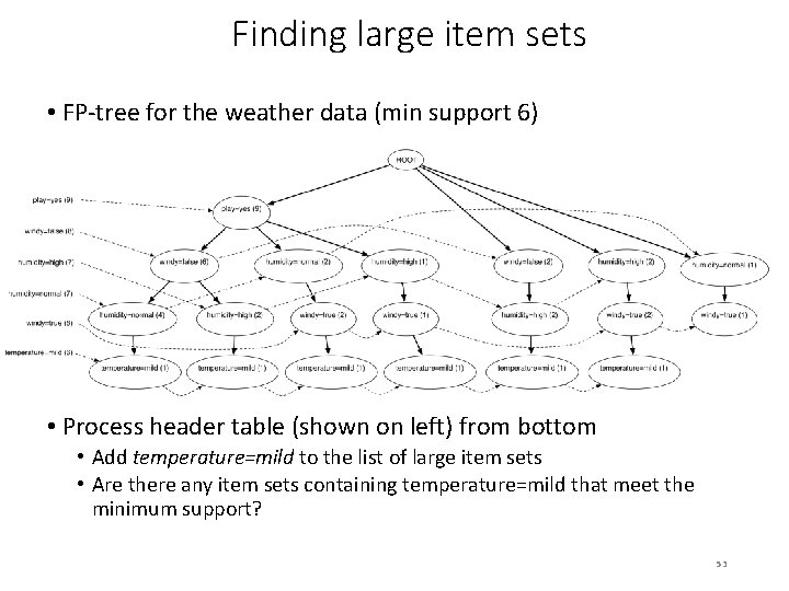
Finding large item sets • FP-tree for the weather data (min support 6) • Process header table (shown on left) from bottom • Add temperature=mild to the list of large item sets • Are there any item sets containing temperature=mild that meet the minimum support? 53

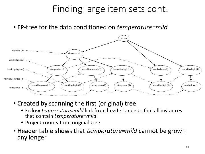
Finding large item sets cont. • FP-tree for the data conditioned on temperature=mild • Created by scanning the first (original) tree • Follow temperature=mild link from header table to find all instances that contain temperature=mild • Project counts from original tree • Header table shows that temperature=mild cannot be grown any longer 54

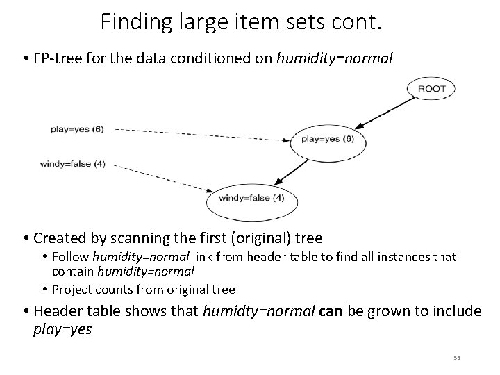
Finding large item sets cont. • FP-tree for the data conditioned on humidity=normal • Created by scanning the first (original) tree • Follow humidity=normal link from header table to find all instances that contain humidity=normal • Project counts from original tree • Header table shows that humidty=normal can be grown to include play=yes 55

Finding large item sets cont. • All large item sets have now been found • However, in order to be sure it is necessary to process the entire header link table from the original tree • Association rules are formed from large item sets in the same way as for Apriori • FP-growth can be up to an order of magnitude faster than Apriori for finding large item sets 56

Discussion and Bibliographic Notes • The FP-tree and the FP-growth algorithm were introduced by Han et al. (2000) following pioneering work by Zaki et al. (1997) • Han et al. (2004) give a more comprehensive description; the algorithm has been extended in various ways • Wang et al. (2003) develop an algorithm called CLOSET+ to mine closed item sets • Close item sets are sets for which there is no proper superset that has the same support • Produces few redundant rules and thus eases the task that users face when examining the output of the mining process • GSP, for Generalized Sequential Patterns, is a method for mining patterns in event sequences (Srikant and Agrawal, 1996) • An approach like FP-growth is used for event sequences by Prefix. Span (Pei et al. , 2004) and Clo. Span (Yan et al. , 2003) • For graph patterns, there is g. Span (Yan and Han, 2002) and Close. Graph (Yan and Han, 2003) 57