Data Mining Nearest Neighbor Classifiers Last Modified 2172019

Data Mining Nearest Neighbor Classifiers Last Modified 2/17/2019 1

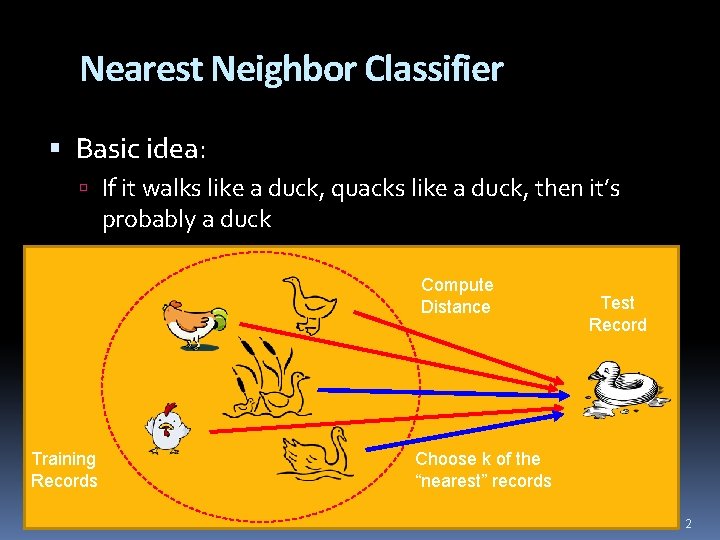
Nearest Neighbor Classifier Basic idea: If it walks like a duck, quacks like a duck, then it’s probably a duck Compute Distance Training Records Test Record Choose k of the “nearest” records 2

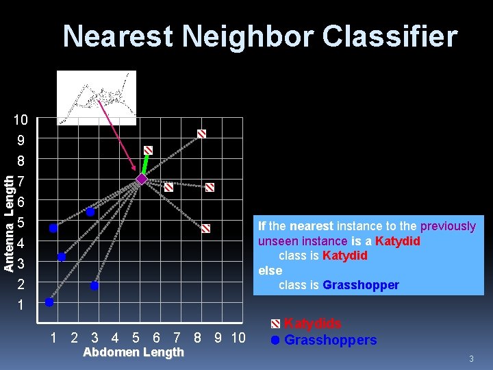
Nearest Neighbor Classifier Antenna Length 10 9 8 7 6 5 4 3 2 1 If the nearest instance to the previously unseen instance is a Katydid class is Katydid else class is Grasshopper 1 2 3 4 5 6 7 8 9 10 Abdomen Length Katydids Grasshoppers 3

Different Learning Methods Eager Learning Explicit description of target function on the whole training set Pretty much all methods we will discuss except this one Lazy Learner Nearest neighbor �also knows as instance-based learning Learning phase=storing all training instances �No “real” work done at learning time Classification=computing distances and determining classification 4

Instance-Based Classifiers Examples: Rote-learner �Memorizes entire training data and performs classification only if attributes of record exactly match one of the training examples �No generalization Nearest neighbor �Uses k “closest” points (nearest neighbors) for performing classification �Generalizes (as do all other methods we cover) 5

Nearest-Neighbor Classifiers l Requires three things – The set of stored records – Distance metric to compute distance between records – The value of k, the number of nearest neighbors to retrieve l To classify an unknown record: – Compute distance to other training records – Identify k nearest neighbors – Use class labels of nearest neighbors to determine the class label of unknown record (e. g. , by taking majority vote) 6

Similarity and Distance One of the fundamental concepts of data mining is the notion of similarity between data points, often formulated as a numeric distance between data points Similarity is the basis for many data mining procedures Covered in our discussion of data 7

k. NN learning Assumes X = n-dim. space discrete or continuous f(x) Nearest neighbor can be used for regression tasks as well as classification tasks �For regression just compute a number based on the numbers associated with the nearest neighbors (e. g. , average) Let x = <a 1(x), …, an(x)> d(xi, xj) = Euclidean distance Algorithm (given new x) find k nearest stored xi (use d(x, xi)) take the most common value of f 8

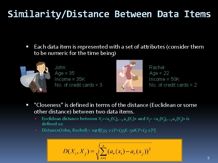
Similarity/Distance Between Data Items Each data item is represented with a set of attributes (consider them to be numeric for the time being) John: Age = 35 Income = 35 K No. of credit cards = 3 Rachel: Age = 22 Income = 50 K No. of credit cards = 2 “Closeness” is defined in terms of the distance (Euclidean or some other distance) between two data items. Euclidean distance between Xi=<a 1(Xi), …, an(Xi)> and Xj= <a 1(Xj), …, an(Xj)> is defined as: Distance(John, Rachel) = sqrt[(35 -22)2+(35 K-50 K)2+(3 -2)2] 9

k-Nearest Neighbor Classifier Example (k=3) Customer Age Income (K) No. of cards Response John 35 35 3 Yes sqrt[(35 -37)22+(35 -50)22 +(3 -2)22]=15. 16 Rachel 22 50 2 No sqrt[(22 -37)22+(50 -50)22 +(2 -2)22]=15 Ruth 63 200 1 No sqrt [(63 -37) 2+(200 -50) 2 +(1 -2) 2]=152. 23 Tom 59 170 1 No sqrt [(59 -37) 2+(170 -50) 2 +(1 -2) 2]=122 Neil 25 40 4 Yes sqrt[(25 -37)22+(40 -50)22 +(4 -2)22]=15. 74 David 37 50 2 ? Yes Distance from David 10

Strengths and Weaknesses Strengths: Quick to build model (essentially no training time) Comprehensible – easy to explain prediction Robust to noisy data by averaging k-nearest neighbors (k not small) Distance function can be tailored using domain knowledge Can learn complex decision boundaries �Much more expressive than linear classifiers & decision trees � More on this later Weaknesses: Need a lot of space to store all examples Takes much more time to classify a new example than with a parsimonious model (need to compare distance to all other examples) Distance function must be designed carefully with domain knowledge �Missing values and irrelevant features are a problem �If done poorly may get bad results 11

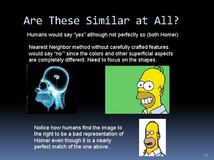
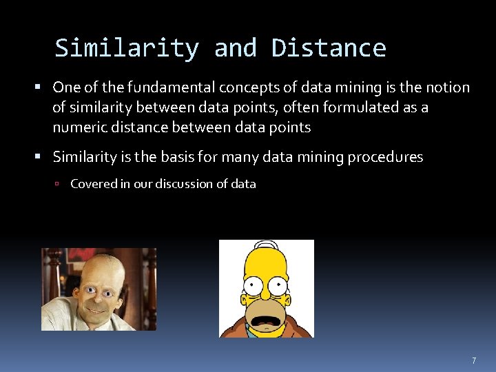
Are These Similar at All? Humans would say “yes” although not perfectly so (both Homer) Nearest Neighbor method without carefully crafted features would say “no’” since the colors and other superficial aspects are completely different. Need to focus on the shapes. Notice how humans find the image to the right to be a bad representation of Homer even though it is a nearly perfect match of the one above. 12

Problems with Computing Similarity Computing similarity is not simple because various factors can interfere These were already covered to some degree in the discussion of “Data” and do not relate only to nearest neighbor- they relate to any method that uses similarity 13

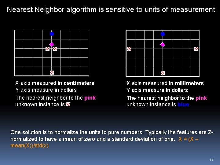
Nearest Neighbor algorithm is sensitive to units of measurement X axis measured in centimeters Y axis measure in dollars The nearest neighbor to the pink unknown instance is X axis measured in millimeters Y axis measure in dollars The nearest neighbor to the pink unknown instance is blue. One solution is to normalize the units to pure numbers. Typically the features are Znormalized to have a mean of zero and a standard deviation of one. X = (X – mean(X))/std(x) 14

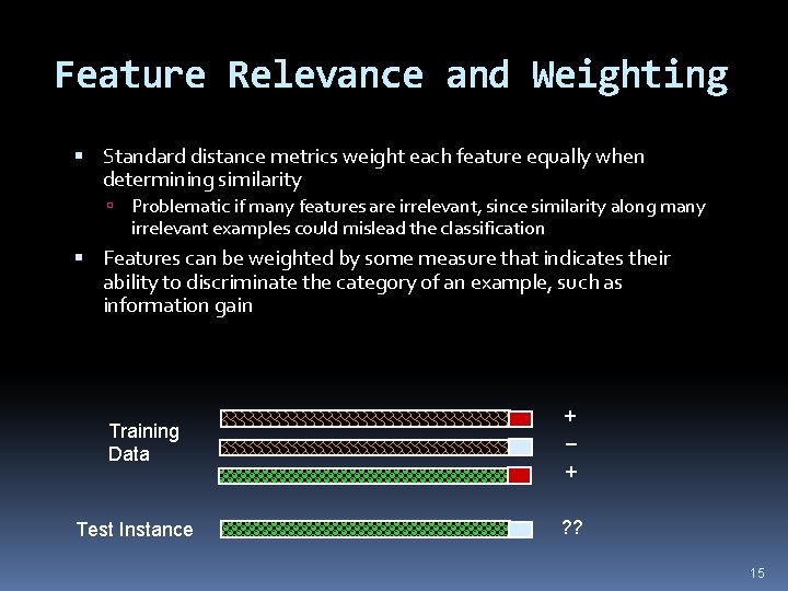
Feature Relevance and Weighting Standard distance metrics weight each feature equally when determining similarity Problematic if many features are irrelevant, since similarity along many irrelevant examples could mislead the classification Features can be weighted by some measure that indicates their ability to discriminate the category of an example, such as information gain Training Data Test Instance + – + ? ? 15

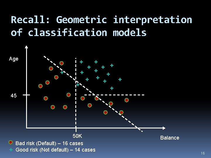
Recall: Geometric interpretation of classification models Age + + + + 45 + 50 K Bad risk (Default) – 16 cases Good risk (Not default) – 14 cases Balance 16

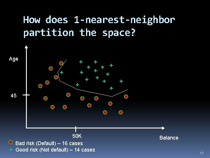
How does 1 -nearest-neighbor partition the space? Age + + + + 45 + 50 K Bad risk (Default) – 16 cases Good risk (Not default) – 14 cases Balance 17

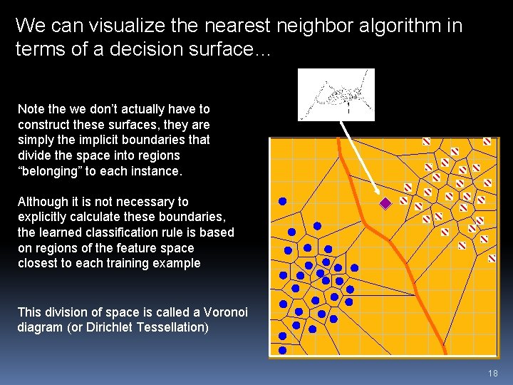
We can visualize the nearest neighbor algorithm in terms of a decision surface… Note the we don’t actually have to construct these surfaces, they are simply the implicit boundaries that divide the space into regions “belonging” to each instance. Although it is not necessary to explicitly calculate these boundaries, the learned classification rule is based on regions of the feature space closest to each training example This division of space is called a Voronoi diagram (or Dirichlet Tessellation) 18

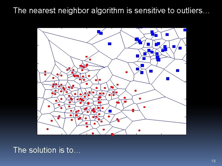
The nearest neighbor algorithm is sensitive to outliers… The solution is to… 19

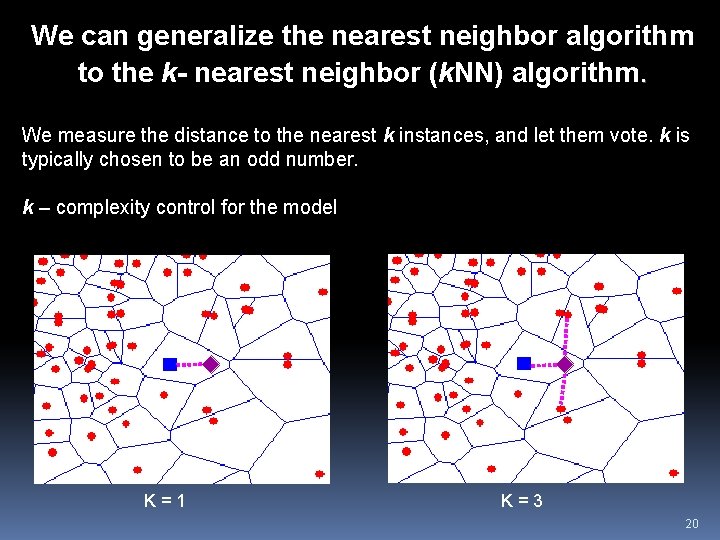
We can generalize the nearest neighbor algorithm to the k- nearest neighbor (k. NN) algorithm. We measure the distance to the nearest k instances, and let them vote. k is typically chosen to be an odd number. k – complexity control for the model K=1 K=3 20

Curse of Dimensionality If each example is described by 20 attributes out of which only 2 are relevant in determining the classification of the target function Then instances that have identical values for the 2 relevant attributes may nevertheless be distant from one another in the 20 dimensional instance space. Having many dimensions complicates the problem and provides more opportunity for problems with irrelevant features or bad distance metrics 21

How to Mitigate Irrelevant Features? Use more training instances Makes it harder to obscure patterns Ask an expert which features are relevant and irrelevant and possibly weight them Use statistical tests (prune irrelevant features) Search over feature subsets 22

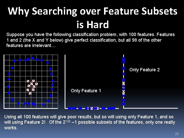
Why Searching over Feature Subsets is Hard Suppose you have the following classification problem, with 100 features. Features 1 and 2 (the X and Y below) give perfect classification, but all 98 of the other features are irrelevant… Only Feature 2 Only Feature 1 Using all 100 features will give poor results, but so will using only Feature 1, and so will using Feature 2! Of the 2100 – 1 possible subsets of the features, only one really works. 23

Nearest Neighbor Variations Can be used to estimate the value of a real-valued function (regression) Take average value of the k nearest neighbors Weight each nearest neighbor’s “vote” by the inverse square of its distance from the test instance More similar examples count more 24

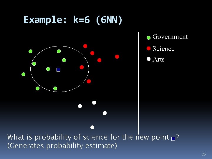
Example: k=6 (6 NN) Government Science Arts What is probability of science for the new point ? (Generates probability estimate) 25

Case-based Reasoning (CBR) CBR is similar to instance-based learning But may reason about the differences between the new example and match example CBR Systems are used a lot help-desk systems legal advice planning & scheduling problems Next time you are on the help with tech support �The person maybe asking you questions based on prompts from a computer program that is trying to most efficiently match you to an existing case! �Feature values are not initially available, you need to ask questions 26

Summary of Pros and Cons Pros: No learning time (lazy learner) Highly expressive since can learn complex decision boundaries Via use of k can avoid noise Easy to explain/justify decision Cons: Relatively long evaluation time No model to provide “high level” insight Very sensitive to irrelevant and redundant features Good distance measures required to get good results 27