DATA MINING Module Nearest Neighbor Classifiers Last modified

DATA MINING Module: Nearest Neighbor Classifiers Last modified 9/27/20 Gary M. Weiss, CIS Dept, Fordham University 1

Nearest-Neighbor Classifiers Basics: How operates and terminology Issues measuring similarity via distance Expressiveness of nearest-neighbor Nearest Neighbor In Practice (Python) Characteristics and Pros and Cons Gary M. Weiss, CIS Dept, Fordham University 2

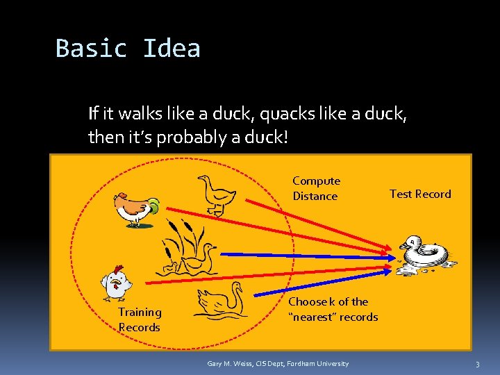
Basic Idea If it walks like a duck, quacks like a duck, then it’s probably a duck! Compute Distance Training Records Test Record Choose k of the “nearest” records Gary M. Weiss, CIS Dept, Fordham University 3

Instance-Based Classifiers Rote-learner Memorizes training data and assign classification only if attributes exactly match a training example No generalization Nearest neighbor Uses k “closest” points (nearest neighbors) for performing classification Generalizes (as do all other methods we cover) Nearest neighbor often used interchangeably with instance-based Gary M. Weiss, CIS Dept, Fordham University 4

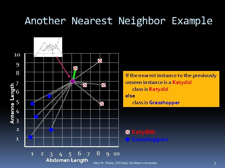
Another Nearest Neighbor Example Antenna Length 10 9 8 7 6 5 4 3 2 1 If the nearest instance to the previously unseen instance is a Katydid class is Katydid else class is Grasshopper Katydids Grasshoppers 1 2 3 4 5 6 7 Abdomen Length 8 9 10 Gary M. Weiss, CIS Dept, Fordham University 5

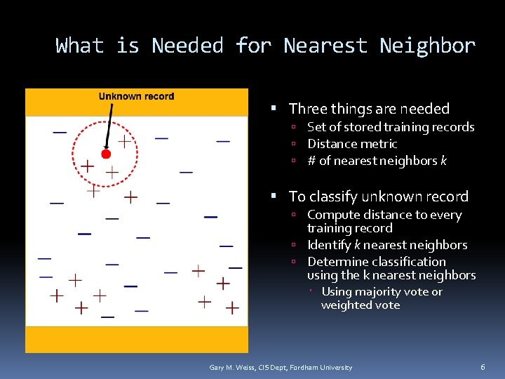
What is Needed for Nearest Neighbor Three things are needed Set of stored training records Distance metric # of nearest neighbors k To classify unknown record Compute distance to every training record Identify k nearest neighbors Determine classification using the k nearest neighbors Using majority vote or weighted vote Gary M. Weiss, CIS Dept, Fordham University 6

Nearest Neighbor is Lazy Learner Most Learners are Eager Work is done up-front Generate an explicit description of target function That is build a model from the training data Lazy Learner Does not build a model: work is deferred Learning phase Just store the training data Testing Phase Essentially all work is done when classifying the example. No explicit model but rather implicit in the data and metrics Gary M. Weiss, CIS Dept, Fordham University 7

Issues With Measuring Similarity Previously covered in “Data” module The issues discussed then also apply now Irrelevant and redundant features are problematic �They throw off the similarity metric �Probably want to remove irrelevant or redundant features using feature selection Different scales and ranges are a problem �Important to normalize the features Differing feature importance is also a problem �Similarity metrics by default weight each feature equally Gary M. Weiss, CIS Dept, Fordham University 8

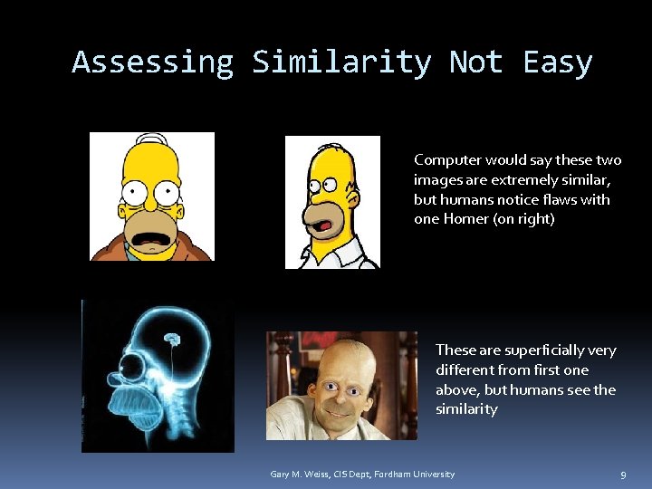
Assessing Similarity Not Easy Computer would say these two images are extremely similar, but humans notice flaws with one Homer (on right) These are superficially very different from first one above, but humans see the similarity Gary M. Weiss, CIS Dept, Fordham University 9

Issues with Different Scales Examples below described by 3 numeric features John: Age = 35 Income = 35, 000 No. of credit cards = 3 Rachel: Age = 22 Income = 50, 000 No. of credit cards = 2 “Closeness” defined in terms of the distance Euclidean distance: square root of sum of the squared differences Distance(John, Rachel) = sqrt[(35 -22)2+(35 K-50 K)2+(3 -2)2] Problem: income dominates due to scale Solution: rescale features to uniform range Gary M. Weiss, CIS Dept, Fordham University 10

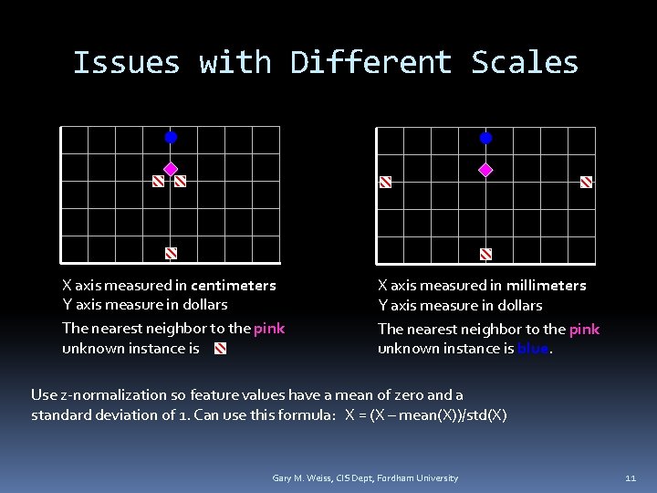
Issues with Different Scales X axis measured in centimeters Y axis measure in dollars The nearest neighbor to the pink unknown instance is X axis measured in millimeters Y axis measure in dollars The nearest neighbor to the pink unknown instance is blue. Use z-normalization so feature values have a mean of zero and a standard deviation of 1. Can use this formula: X = (X – mean(X))/std(X) Gary M. Weiss, CIS Dept, Fordham University 11

Irrelevant Features If each example described by 20 attributes but only 2 are relevant Examples with identical values for the 2 attributes may still be distant in 20 -dimensional instance space How to mitigate irrelevant features? Use more training instances Harder to obscure patterns Ask an expert which features are irrelevant and drop Use statistical tests (prune irrelevant features) Search feature subsets as covered in “Data” module Gary M. Weiss, CIS Dept, Fordham University 12

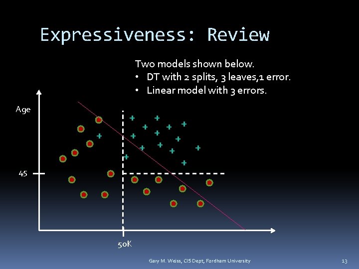
Expressiveness: Review Two models shown below. • DT with 2 splits, 3 leaves, 1 error. • Linear model with 3 errors. Age + + 45 + + + + 50 K Gary M. Weiss, CIS Dept, Fordham University 13

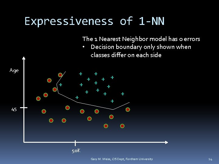
Expressiveness of 1 -NN The 1 Nearest Neighbor model has 0 errors • Decision boundary only shown when classes differ on each side Age + + + + 45 50 K Gary M. Weiss, CIS Dept, Fordham University 14

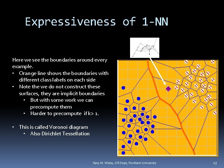
Expressiveness of 1 -NN Here we see the boundaries around every example. • Orange line shows the boundaries with different class labels on each side • Note the we do not construct these surfaces, they are implicit boundaries • But with some work we can precompute them • Harder to precompute if k> 1. • This is called Voronoi diagram • Also Dirichlet Tessellation Gary M. Weiss, CIS Dept, Fordham University 15

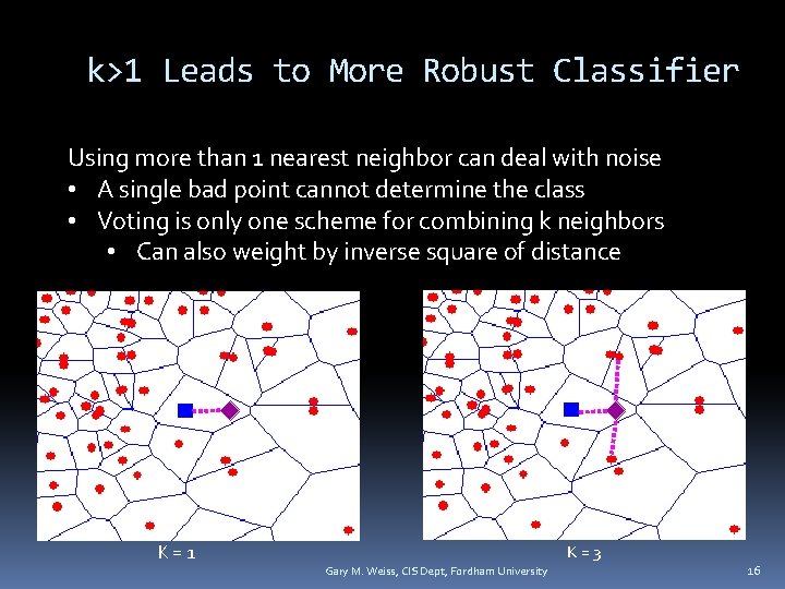
k>1 Leads to More Robust Classifier Using more than 1 nearest neighbor can deal with noise • A single bad point cannot determine the class • Voting is only one scheme for combining k neighbors • Can also weight by inverse square of distance K=1 K=3 Gary M. Weiss, CIS Dept, Fordham University 16

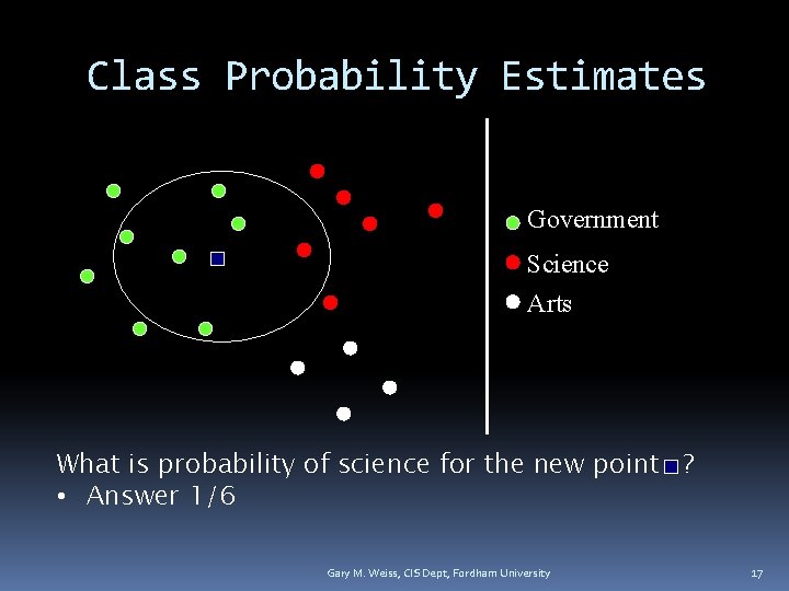
Class Probability Estimates Government Science Arts What is probability of science for the new point ? • Answer 1/6 Gary M. Weiss, CIS Dept, Fordham University 17

Handling Regression Tasks Nearest neighbor can be used to predict numbers How? Take average or median value of k nearest neighbors Weight values by inverse square of its distance from the test instance Gary M. Weiss, CIS Dept, Fordham University 18

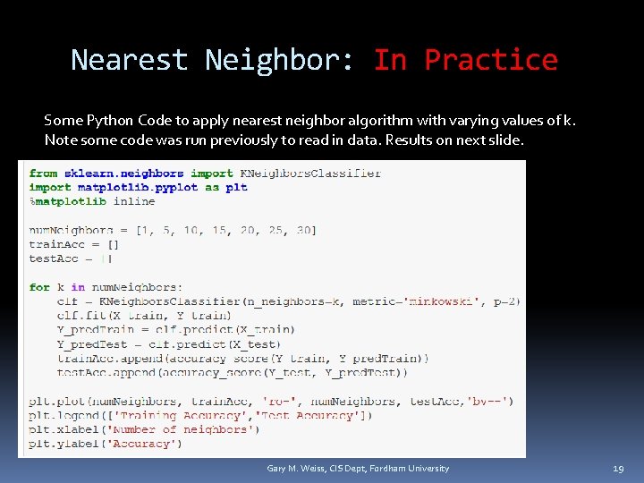
Nearest Neighbor: In Practice Some Python Code to apply nearest neighbor algorithm with varying values of k. Note some code was run previously to read in data. Results on next slide. Gary M. Weiss, CIS Dept, Fordham University 19

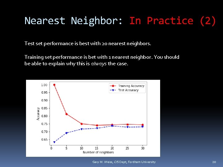
Nearest Neighbor: In Practice (2) Test set performance is best with 20 nearest neighbors. Training set performance is bet with 1 nearest neighbor. You should be able to explain why this is always the case. Gary M. Weiss, CIS Dept, Fordham University 20

Summary of k. NN Pros and Cons Pros: Quick training (no learning time-lazy learner) Easy to explain/justify decision Robust to noise (choose k > 1) Very expressive- highly complex decision boundaries Can also be used for regression tasks Cons: Relatively long evaluation time Need to save all training examples No model to provide “high level” insight Sensitive to irrelevant and redundant features Need to carefully engineer distance metric Gary M. Weiss, CIS Dept, Fordham University 21