Data Mining Metode dan Algoritma Romi Satria Wahono

Data Mining: Metode dan Algoritma Romi Satria Wahono romi@romisatriawahono. net http: //romisatriawahono. net 0815 -86220090

Romi Satria Wahono § SD Sompok Semarang (1987) § SMPN 8 Semarang (1990) § SMA Taruna Nusantara, Magelang (1993) § S 1, S 2 dan S 3 (on-leave) Department of Computer Sciences Saitama University, Japan (1994 -2004) § Research Interests: Software Engineering and Intelligent Systems § Founder Ilmu. Komputer. Com § Peneliti LIPI (2004 -2009) § Founder dan CEO PT Brainmatics Cipta Informatika

Course Outline 1. Pengenalan Data Mining 2. Proses Data Mining 3. Evaluasi dan Validasi pada Data Mining 4. Metode dan Algoritma Data Mining 5. Penelitian Data Mining

Metode dan Algoritma

Metode dan Algoritma 1. Inferring rudimentary rules 2. Statistical modeling 3. Constructing decision trees 4. Constructing rules 5. Association rule learning 6. Linear models 7. Instance-based learning 8. Clustering

Simplicity first § Simple algorithms often work very well! § There are many kinds of simple structure, eg: • One attribute does all the work • All attributes contribute equally & independently • A weighted linear combination might do • Instance-based: use a few prototypes • Use simple logical rules § Success of method depends on the domain

Inferring rudimentary rules § 1 R: learns a 1 -level decision tree • I. e. , rules that all test one particular attribute § Basic version • One branch for each value • Each branch assigns most frequent class • Error rate: proportion of instances that don’t belong to the majority class of their corresponding branch • Choose attribute with lowest error rate (assumes nominal attributes)

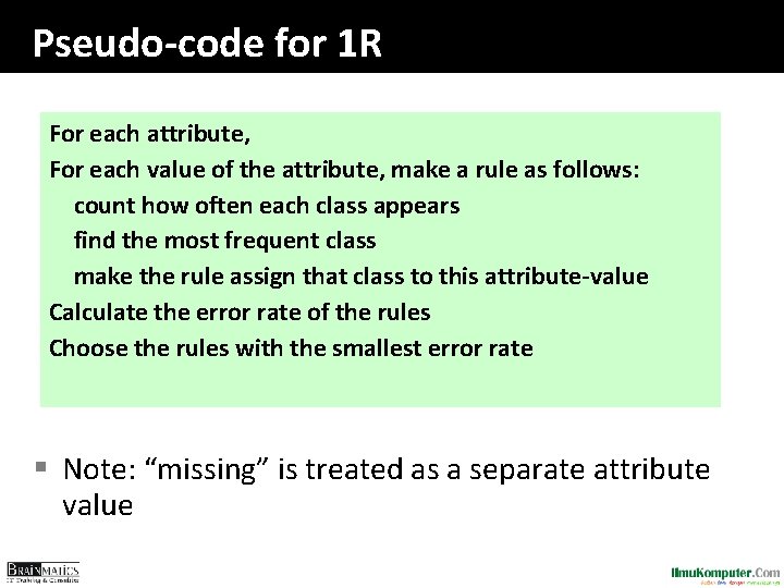
Pseudo-code for 1 R For each attribute, For each value of the attribute, make a rule as follows: count how often each class appears find the most frequent class make the rule assign that class to this attribute-value Calculate the error rate of the rules Choose the rules with the smallest error rate § Note: “missing” is treated as a separate attribute value

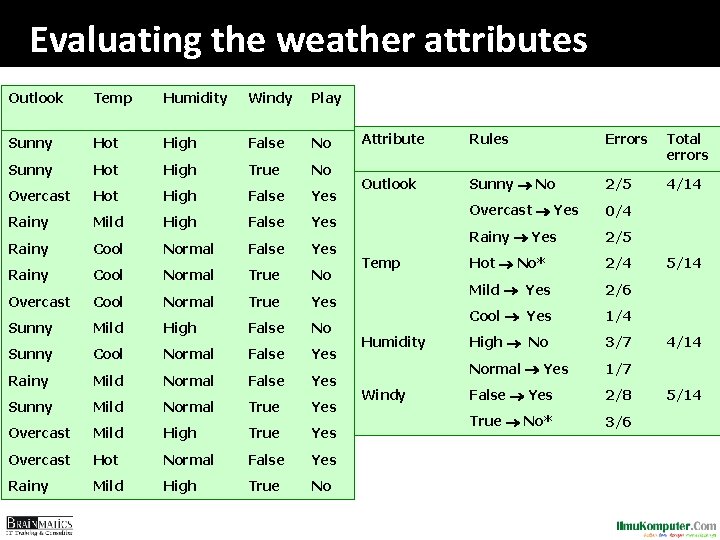
Evaluating the weather attributes Outlook Temp Humidity Windy Play Sunny Hot High False No Sunny Hot High True No Overcast Hot High False Yes Rainy Mild High False Yes Rainy Cool Normal True No Overcast Cool Normal True Yes Sunny Mild High False No Sunny Cool Normal False Yes Rainy Mild Normal False Yes Sunny Mild Normal True Yes Overcast Mild High True Yes Overcast Hot Normal False Yes Rainy Mild High True No Attribute Rules Errors Total errors Outlook Sunny No 2/5 4/14 Overcast Yes 0/4 Rainy Yes 2/5 Hot No* 2/4 Mild Yes 2/6 Cool Yes 1/4 High No 3/7 Normal Yes 1/7 False Yes 2/8 True No* 3/6 Temp Humidity Windy 5/14 4/14 5/14

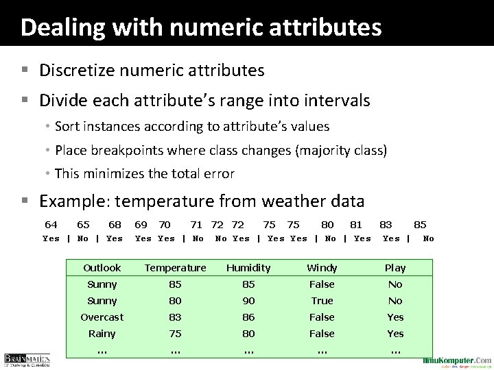
Dealing with numeric attributes § Discretize numeric attributes § Divide each attribute’s range into intervals • Sort instances according to attribute’s values • Place breakpoints where class changes (majority class) • This minimizes the total error § Example: temperature from weather data 64 65 68 Yes | No | Yes 69 70 71 72 72 75 75 80 81 83 85 Yes | No No Yes | Yes Yes | No Outlook Temperature Humidity Windy Play Sunny 85 85 False No Sunny 80 90 True No Overcast 83 86 False Yes Rainy 75 80 False Yes … … …

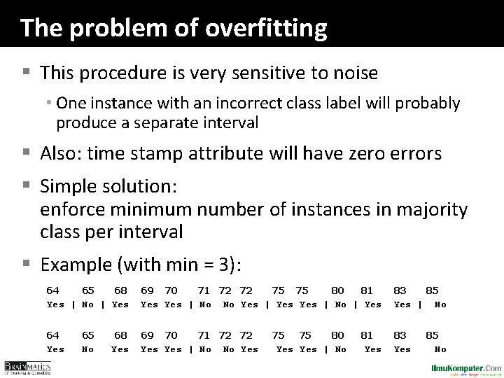
The problem of overfitting § This procedure is very sensitive to noise • One instance with an incorrect class label will probably produce a separate interval § Also: time stamp attribute will have zero errors § Simple solution: enforce minimum number of instances in majority class per interval § Example (with min = 3): 64 65 68 Yes | No | Yes 69 70 71 72 72 75 75 80 81 Yes | No No Yes | No | Yes 83 85 Yes | No 64 Yes 69 70 71 72 72 Yes | No No Yes 83 Yes 65 No 68 Yes 75 75 80 Yes | No 81 Yes 85 No

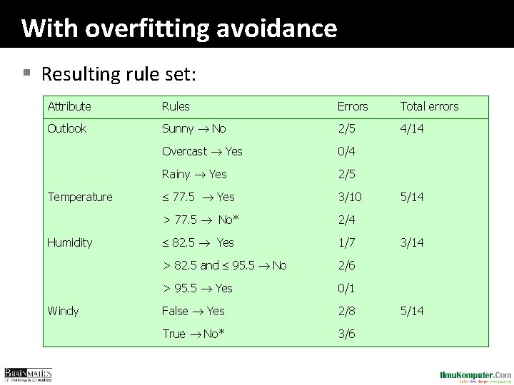
With overfitting avoidance § Resulting rule set: Attribute Rules Errors Total errors Outlook Sunny No 2/5 4/14 Overcast Yes 0/4 Rainy Yes 2/5 77. 5 Yes 3/10 > 77. 5 No* 2/4 82. 5 Yes 1/7 > 82. 5 and 95. 5 No 2/6 > 95. 5 Yes 0/1 False Yes 2/8 True No* 3/6 Temperature Humidity Windy 5/14 3/14 5/14

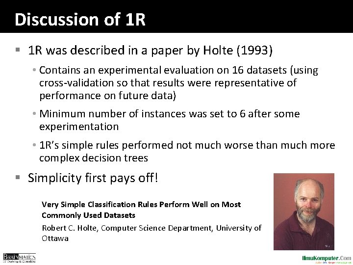
Discussion of 1 R § 1 R was described in a paper by Holte (1993) • Contains an experimental evaluation on 16 datasets (using cross-validation so that results were representative of performance on future data) • Minimum number of instances was set to 6 after some experimentation • 1 R’s simple rules performed not much worse than much more complex decision trees § Simplicity first pays off! Very Simple Classification Rules Perform Well on Most Commonly Used Datasets Robert C. Holte, Computer Science Department, University of Ottawa

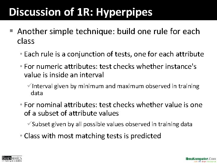
Discussion of 1 R: Hyperpipes § Another simple technique: build one rule for each class • Each rule is a conjunction of tests, one for each attribute • For numeric attributes: test checks whether instance's value is inside an interval üInterval given by minimum and maximum observed in training data • For nominal attributes: test checks whether value is one of a subset of attribute values üSubset given by all possible values observed in training data • Class with most matching tests is predicted

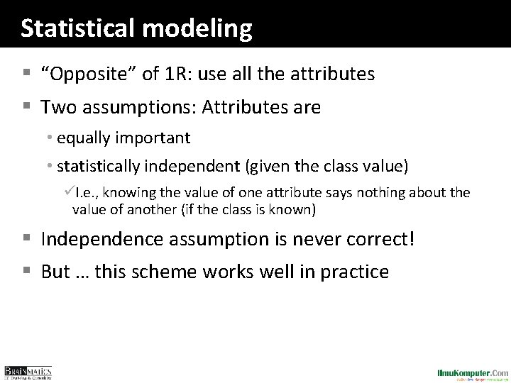
Statistical modeling § “Opposite” of 1 R: use all the attributes § Two assumptions: Attributes are • equally important • statistically independent (given the class value) üI. e. , knowing the value of one attribute says nothing about the value of another (if the class is known) § Independence assumption is never correct! § But … this scheme works well in practice

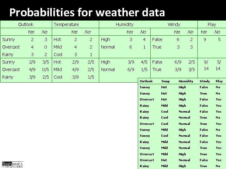
Probabilities for weather data Outlook Temperature Yes Humidity Yes No No Sunny 2 3 Hot 2 2 Overcast 4 0 Mild 4 2 Rainy 3 2 Cool 3 1 Sunny 2/9 3/5 Hot 2/9 2/5 Overcast 4/9 0/5 Mild 4/9 2/5 Rainy 3/9 2/5 Cool 3/9 1/5 Windy Yes No High 3 4 Normal 6 High Normal Play Yes No False 6 2 9 5 1 True 3 3 3/9 4/5 False 6/9 2/5 6/9 1/5 True 3/9 3/5 9/ 14 5/ 14 Outlook Temp Humidity Windy Play Sunny Hot High False No Sunny Hot High True No Overcast Hot High False Yes Rainy Mild High False Yes Rainy Cool Normal True No Overcast Cool Normal True Yes Sunny Mild High False No Sunny Cool Normal False Yes Rainy Mild Normal False Yes Sunny Mild Normal True Yes Overcast Mild High True Yes Overcast Hot Normal False Yes Rainy Mild High True No

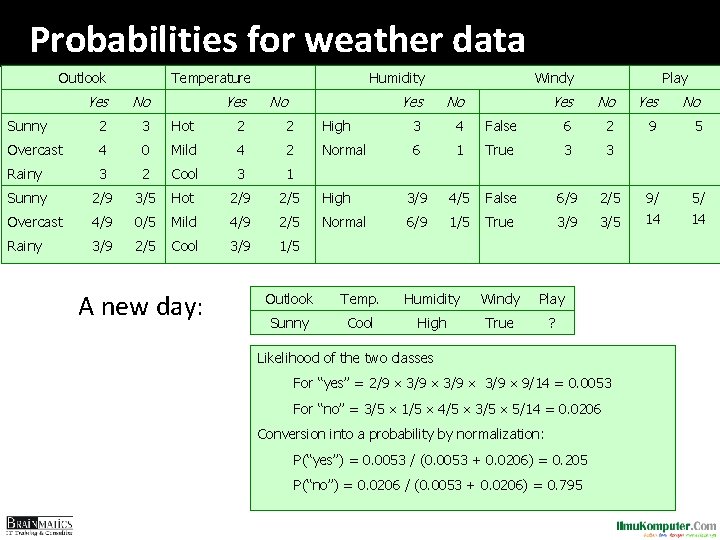
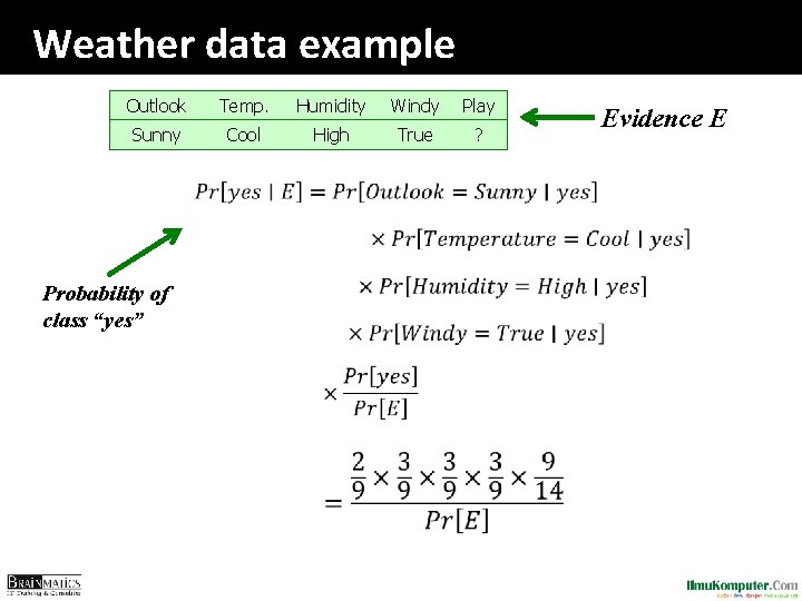
Probabilities for weather data Outlook Temperature Yes Humidity Yes No Sunny 2 3 Hot 2 2 Overcast 4 0 Mild 4 2 Rainy 3 2 Cool 3 1 Sunny 2/9 3/5 Hot 2/9 2/5 Overcast 4/9 0/5 Mild 4/9 2/5 Rainy 3/9 2/5 Cool 3/9 1/5 A new day: No Windy Yes No High 3 4 Normal 6 High Normal Play Yes No False 6 2 9 5 1 True 3 3 3/9 4/5 False 6/9 2/5 6/9 1/5 True 3/9 3/5 9/ 14 5/ 14 Outlook Temp. Humidity Windy Play Sunny Cool High True ? Likelihood of the two classes For “yes” = 2/9 3/9 9/14 = 0. 0053 For “no” = 3/5 1/5 4/5 3/5 5/14 = 0. 0206 Conversion into a probability by normalization: P(“yes”) = 0. 0053 / (0. 0053 + 0. 0206) = 0. 205 P(“no”) = 0. 0206 / (0. 0053 + 0. 0206) = 0. 795

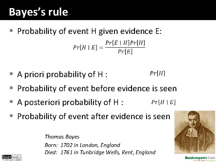
Bayes’s rule § Probability of event H given evidence E: § A priori probability of H : § Probability of event before evidence is seen § A posteriori probability of H : § Probability of event after evidence is seen Thomas Bayes Born: 1702 in London, England Died: 1761 in Tunbridge Wells, Kent, England

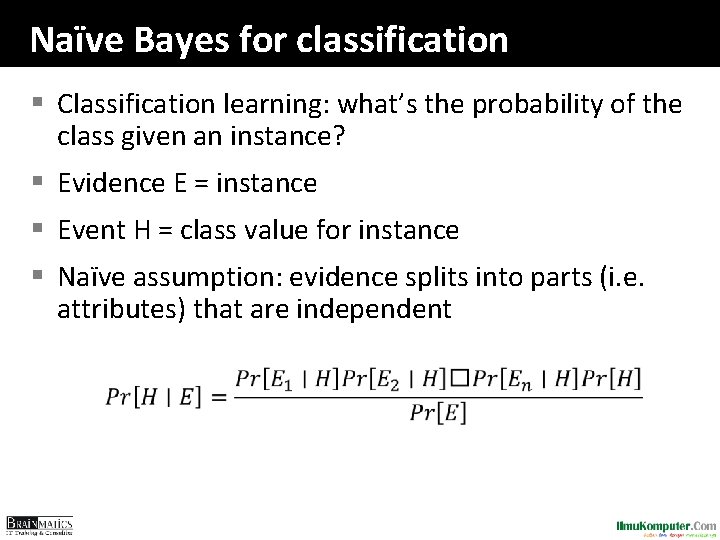
Naïve Bayes for classification § Classification learning: what’s the probability of the class given an instance? § Evidence E = instance § Event H = class value for instance § Naïve assumption: evidence splits into parts (i. e. attributes) that are independent

Weather data example Outlook Temp. Humidity Windy Play Sunny Cool High True ? Probability of class “yes” Evidence E

Cognitive Assignment II § Pahami dan kuasai satu metode data mining dari berbagai literatur § Rangkumkan dengan detail dalam bentuk slide, dari mulai definisi, perkembangan metode, tahapan algoritma, penerapannya untuk suatu studi kasus, dan buat/temukan code Java (eksekusi contoh kasus) § Presentasikan di depan kelas pada mata kuliah berikutnya dengan bahasa manusia

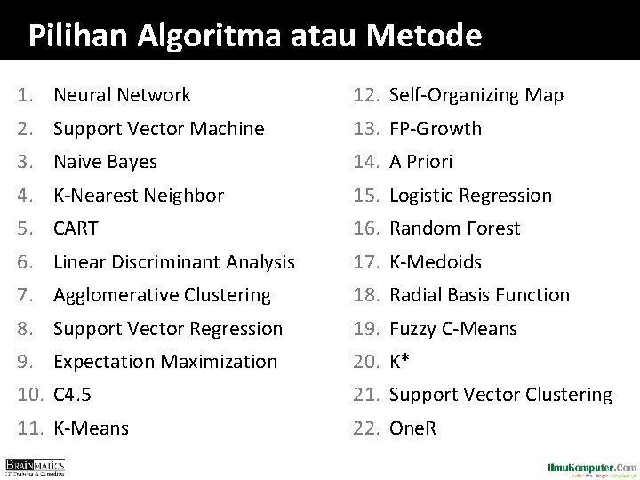
Pilihan Algoritma atau Metode 1. Neural Network 12. Self-Organizing Map 2. Support Vector Machine 13. FP-Growth 3. Naive Bayes 14. A Priori 4. K-Nearest Neighbor 15. Logistic Regression 5. CART 16. Random Forest 6. Linear Discriminant Analysis 17. K-Medoids 7. Agglomerative Clustering 18. Radial Basis Function 8. Support Vector Regression 19. Fuzzy C-Means 9. Expectation Maximization 20. K* 10. C 4. 5 21. Support Vector Clustering 11. K-Means 22. One. R

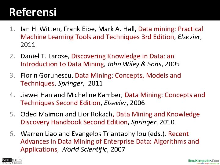
Referensi 1. Ian H. Witten, Frank Eibe, Mark A. Hall, Data mining: Practical Machine Learning Tools and Techniques 3 rd Edition, Elsevier, 2011 2. Daniel T. Larose, Discovering Knowledge in Data: an Introduction to Data Mining, John Wiley & Sons, 2005 3. Florin Gorunescu, Data Mining: Concepts, Models and Techniques, Springer, 2011 4. Jiawei Han and Micheline Kamber, Data Mining: Concepts and Techniques Second Edition, Elsevier, 2006 5. Oded Maimon and Lior Rokach, Data Mining and Knowledge Discovery Handbook Second Edition, Springer, 2010 6. Warren Liao and Evangelos Triantaphyllou (eds. ), Recent Advances in Data Mining of Enterprise Data: Algorithms and Applications, World Scientific, 2007