Data Mining Methods in Web Analysis Kristna Machov

Data Mining Methods in Web Analysis Kristína Machová

Content o Machine learning o Decision trees o Ensemble learning o Bagging o Boosting o Random forests o Applications of machine learning o Sentiment analysis o Authorities and trolls identification

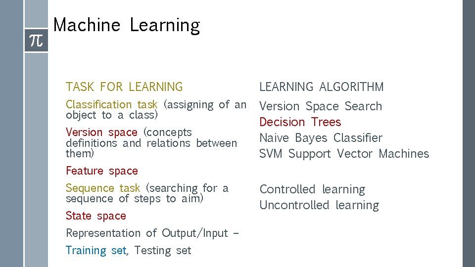
Machine Learning TASK FOR LEARNING ALGORITHM Classification task (assigning of an object to a class) Version Space Search Decision Trees Naive Bayes Classifier SVM Support Vector Machines Version space (concepts definitions and relations between them) Feature space Sequence task (searching for a sequence of steps to aim) State space Representation of Output/Input – Training set, Testing set Controlled learning Uncontrolled learning

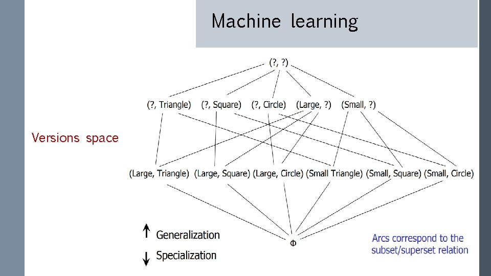
Machine learning Versions space

Machine learning Feature space

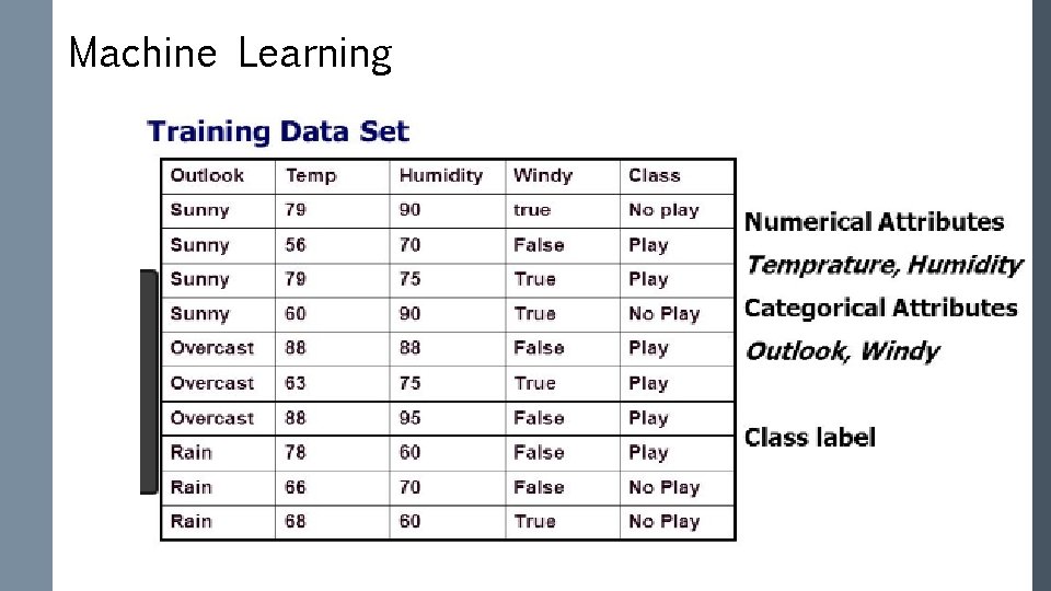
Machine Learning MACHINE LEARNING

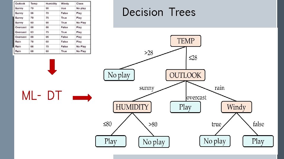
Decision Trees ML- DT

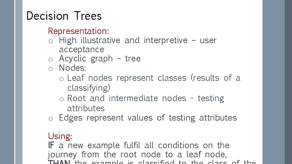
Decision Trees Representation: o High illustrative and interpretive – user acceptance o Acyclic graph – tree o Nodes: o Leaf nodes represent classes (results of a classifying) o Root and intermediate nodes - testing attributes o Edges represent values of testing attributes Using: IF a new example fulfil all conditions on the journey from the root node to a leaf node,

Decision Trees Induction o Application of an approach „Separate and Conquer“ o Ending Condition (EC) o perfect classification – each subspace contains only examples of one – the same class o non-perfect classification - each subspace contains eg. 90% examples of one class o General algorithm: IF EC is fulfil for each subspace THEN End ELSE 1. Choose a subspace with examples of different classes 2. Select still unused testing attribute TA 3. Split the subspace to other subspaces according values of TA

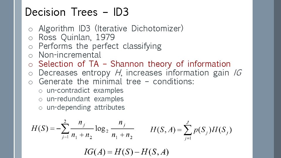
Decision Trees – ID 3 o o o o Algorithm ID 3 (Iterative Dichotomizer) Ross Quinlan, 1979 Performs the perfect classifying Non-incremental Selection of TA – Shannon theory of information Decreases entropy H, increases information gain IG Generate the minimal tree – conditions: o un-contradict examples o un-redundant examples o un-depending attributes

Decision Trees - C 4. 5 Ross Quinlan, 1993 Modification of algorithm ID 3 Non-incremental induction Attributes: o discrete (nominal, binary) o continuous (real, integer numbers) o Ratio Information Gain (IGr) o New possibilities – to process: o continuous attributes o un-known values of attributes o o

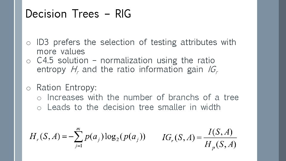
Decision Trees – RIG o ID 3 prefers the selection of testing attributes with more values o C 4. 5 solution – normalization using the ratio entropy Hr and the ratio information gain IGr o Ration Entropy: o Increases with the number of branchs of a tree o Leads to the decision tree smaller in width

Decision Trees – Continuous Attributes o Values of a continuous attribute are ordered o Threshold value is computed for each pair of neighbor values as the arithmetic mean (average) o There are m-1 thresholds for m values of the attribute o We need to select one threshold for dividing space of examples into two sub-spaces o The threshold with maximal ratio information gain IGr is selected o The space is divided into two subspaces according selected threshold: o First subspace - examples with attribute values less then the selected threshold o Second subspace – greater then the threshold

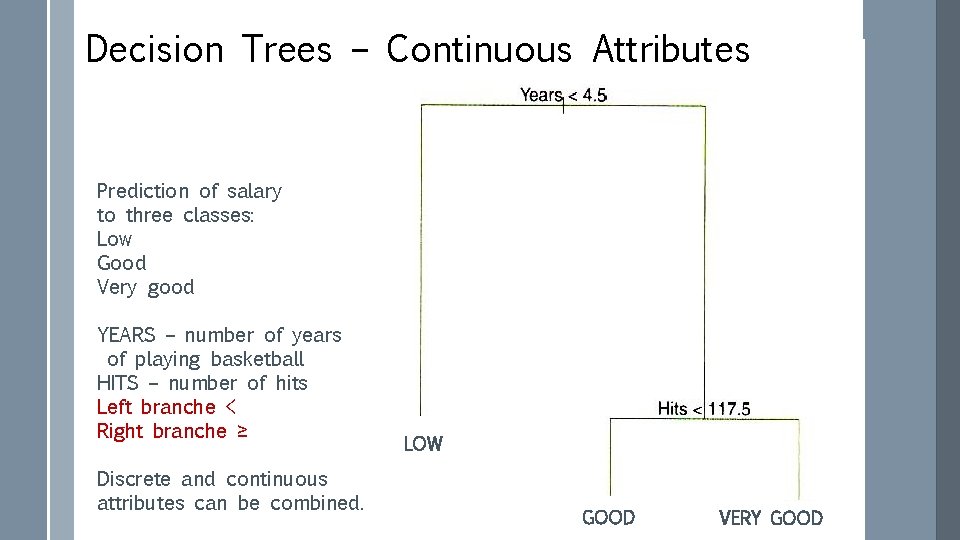
Decision Trees – Continuous Attributes Prediction of salary to three classes: Low Good Very good YEARS – number of years of playing basketball HITS – number of hits Left branche < Right branche ≥ Discrete and continuous attributes can be combined. LOW GOOD VERY GOOD

Ensemble Learning o Too small or less quality training set (irrelevant attributes, non – typical examples of class) o Weak classifier – low effectivity o Various samples of a training set are formed o On each sample, one particular weak classifier is learned o The result classification is created by the voting among all particular classifiers o Stacking o Bagging o Boosting o Random forests

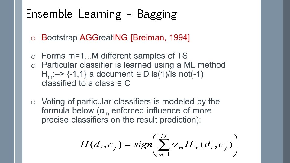
Ensemble Learning – Bagging

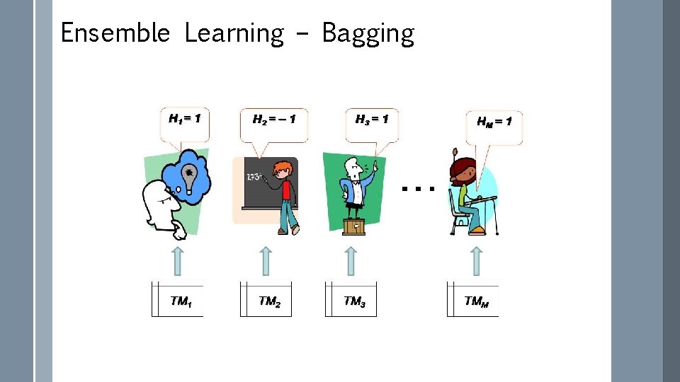
Ensemble Learning – Bagging

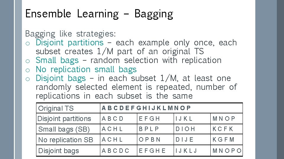
Ensemble Learning – Bagging like strategies: o Disjoint partitions – each example only once, each subset creates 1/M part of an original TS o Small bags – random selection with replication o No replication small bags o Disjoint bags – in each subset 1/M, at least one randomly selected element is repeated, number of replications in each subset is the same Original TS Disjoint partitions Small bags (SB) No replication SB ABCDEFGHIJKLMNOP Disjoint bags ABCD EFGH IJKL MNOP ACHL BPLP DIOH KCFK ACHL OPBN DIJE KGFM ABCDC EFGHE IJKLJ MNOPO

Ensemble Learning – Boosting is an improved bagging [Schapire-Singer, 1999] based on the weighting of training examples o Forms m=1. . . M samples from the original TS o Samples differ only in weights of training examples o On every sample, weak classifier is trained Hm: –> {-1, 1} using the same selected algorithm of ML o In every iteration: o weights of wrong/right classified examples are increased/decreased o modified sample is used for learning of the new classifier o Error driven ensemble learning – better results o Result of classification is the result of voting of particular classifiers (similar as in the bagging)

Ensemble Learning – Random Forests o Random Forests [Breiman, 2001] is a modification of the bagging o EL is based exceptionally on the decision tree ML method o Generates a set of de-correlated trees – forest of trees o Ensemble classifier o averages results of classifying of particular decision trees (regression DT) o creates the result of voting by particular classifiers DTs (classification DT) o Particular classifiers have to be independent (de-correlated) – random selection of a subset of attributes for every tree o Independent trees can be generated in parallel process o Random selection of training subset of training set for generation of every decision tree

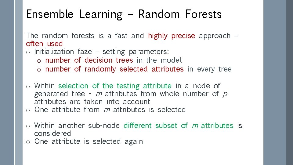
Ensemble Learning – Random Forests The random forests is a fast and highly precise approach – often used o Initialization faze – setting parameters: o number of decision trees in the model o number of randomly selected attributes in every tree o Within selection of the testing attribute in a node of generated tree - m attributes from whole number of p attributes are taken into account o One attribute from m attributes is selected o Within another sub-node different subset of m attributes is considered o One attribute is selected again

Ensemble Learning – Random Forests o Within every splitting of the space of training examples it is forbidden to use some attributes (unselected for subset of m attributes) – Why? Irrational? o IF there is one strong predictor in a group of slightly strong predictors THEN the strong predictor will be used for generation of all trees o Leads to similar trees - strong correlation of the trees o Averaging of the forest of highly correlated trees will not bring any benefit compared to using only one tree o Principle of de-correlation of trees – the probability of the selection of a strong predictor will be only (p-m)/p – other predictors will have more chance

Ensemble Learning – Random Forests o Main difference between the random forest and the bagging is the selection of a subset of m predictors o IF m=p THEN the random forest is equal to the bagging o Less value m leads to a more reliable random forest (mainly in the case of many correlated predictors o It is easier to train the random forest then tune the boosting

Ensemble Learning - Comparison o Ensemble Learning increases the precision of a classification providing a voting of the set of weak classifiers (strong classifier do not need to rejoice) o Cons: o loss of a clarity o result of the learning is less illustrative o increasing of a computational complexity o Achieve results prefer boosting before bagging o Error driven ensemble learning in the boosting not only refines results but also accelerates the learning o Random forests do not require much tuning o They achieve only 4, 88% of the classification error (bagging 5, 4%). o They can not be over-learned

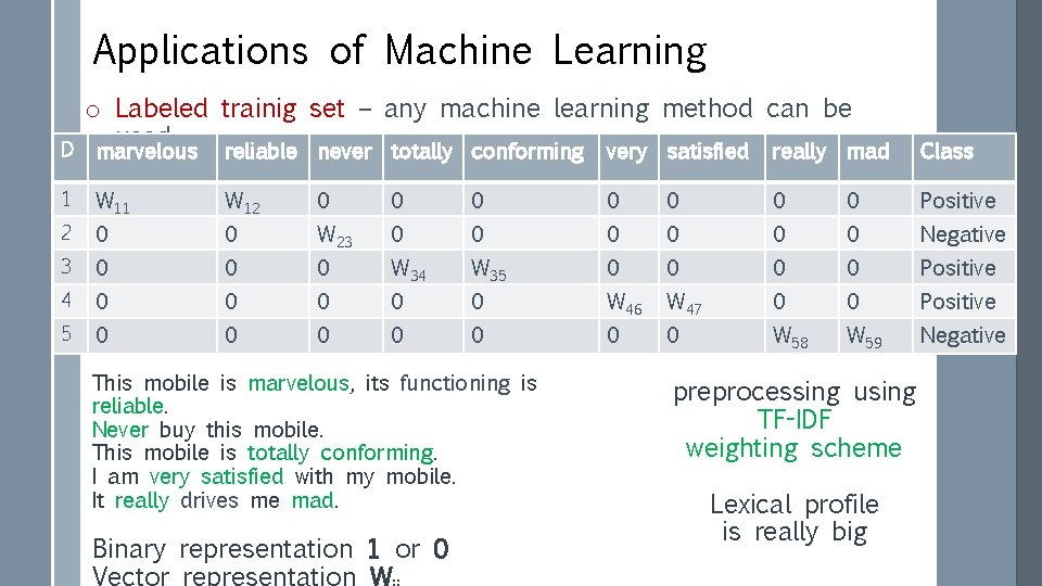
Applications of Machine Learning D o Labeled trainig set – any machine learning method can be used marvelous reliable never totally conforming very satisfied really mad Class 1 W 12 0 0 0 0 Positive 2 0 0 W 23 0 0 0 Negative 3 0 0 0 W 34 W 35 0 0 Positive 4 0 0 0 W 46 W 47 0 0 Positive 5 0 0 0 0 W 58 W 59 Negative This mobile is marvelous, its functioning is reliable. Never buy this mobile. This mobile is totally conforming. I am very satisfied with my mobile. It really drives me mad. Binary representation 1 or 0 preprocessing using TF-IDF weighting scheme Lexical profile is really big

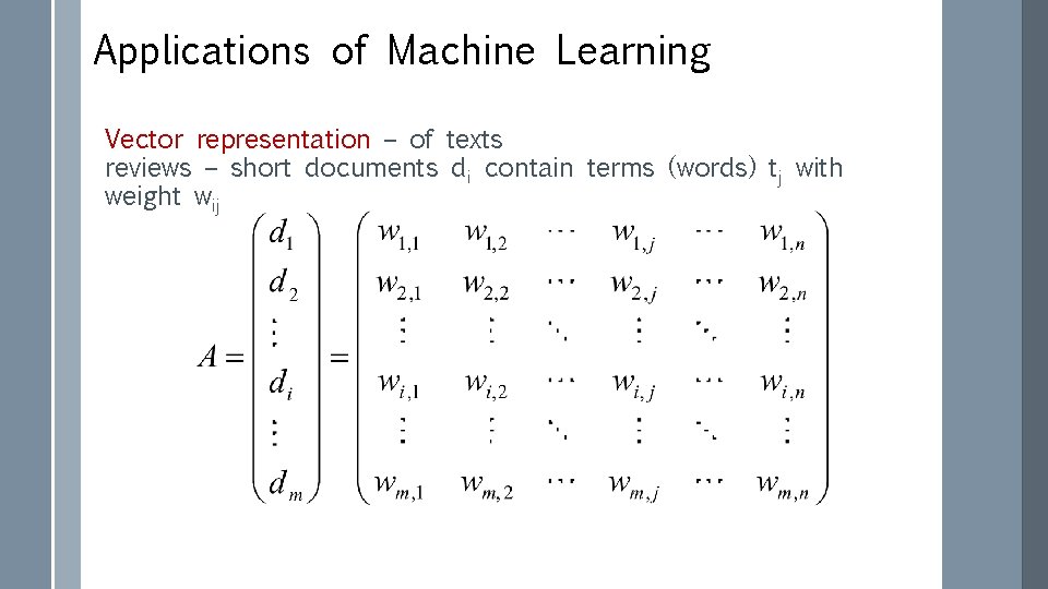
Applications of Machine Learning Vector representation – of texts reviews – short documents di contain terms (words) tj with weight wij

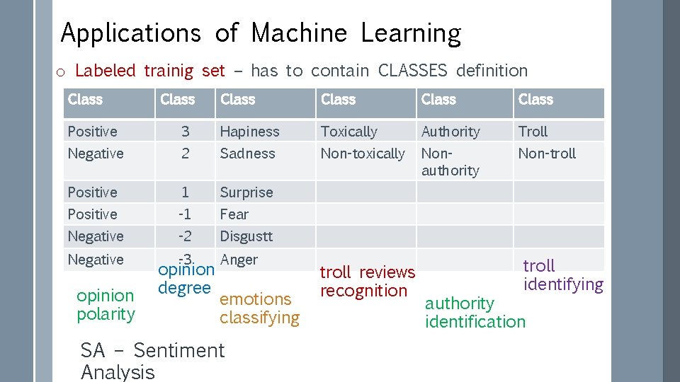
Applications of Machine Learning o Labeled trainig set – has to contain CLASSES definition Class Class Positive 3 Hapiness Toxically Authority Troll Negative 2 Sadness Non-toxically Nonauthority Non-troll Positive 1 Surprise Positive -1 Fear Negative -2 Disgustt Negative -3 Anger opinion polarity opinion degree emotions classifying SA – Sentiment Analysis troll reviews recognition troll identifying authority identification

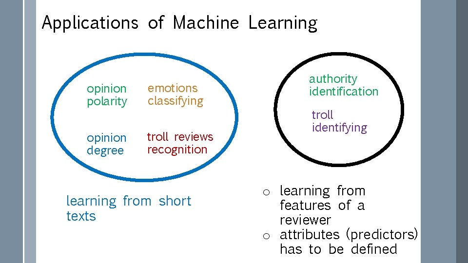
Applications of Machine Learning opinion polarity emotions classifying opinion degree troll reviews recognition learning from short texts authority identification troll identifying o learning from features of a reviewer o attributes (predictors) has to be defined

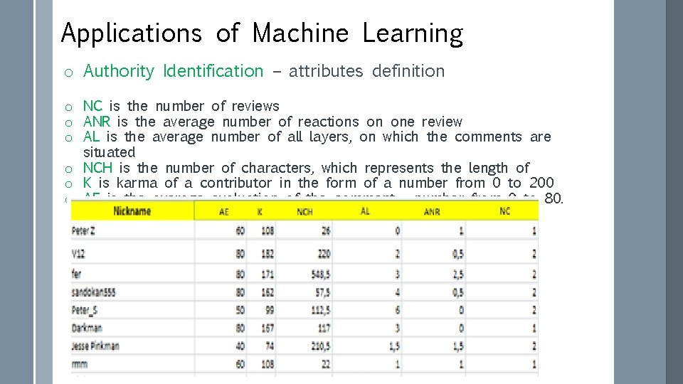
Applications of Machine Learning o Authority Identification – attributes definition o NC is the number of reviews o ANR is the average number of reactions on one review o AL is the average number of all layers, on which the comments are situated o NCH is the number of characters, which represents the length of o K is karma of a contributor in the form of a number from 0 to 200 o AE is the average evaluation of the comment - number from 0 to 80.

Applications of Machine Learning o Troll identifying – attributes definition ? o o o o Abusive troll Insistent troll Troll, who controls the grammar Always injured troll Troll, who knows everything Troll, who is beyond theme Troll, who is a continuous spamer