DATA MINING LINK ANALYSIS RANKING Page Rank Random

.")


: using the web")


 Page. Rank algorithm • Performing vanilla power method is now too expensive")


![Hubs and Authorities [K 98] • Authority is not necessarily transferred directly between authorities](https://slidetodoc.com/presentation_image_h2/8b444cf87efc1969f74df3b330a5a3b9/image-64.jpg "Hubs and Authorities [K 98] • Authority is not necessarily transferred directly between authorities")


 1/3 2/3 1/3 hubs 1 5/6 2/6 1/6")


![Singular Value Decomposition [n×r] [r×n] • r : rank of matrix A • σ1≥](https://slidetodoc.com/presentation_image_h2/8b444cf87efc1969f74df3b330a5a3b9/image-76.jpg "Singular Value Decomposition [n×r] [r×n] • r : rank of matrix A • σ1≥")


 • counts the number of citations received")


 •")


 • The expected number")


- Slides: 115
DATA MINING LINK ANALYSIS RANKING Page. Rank -- Random walks HITS Absorbing Random Walks and Label Propagation
Network Science • A number of complex systems can be modeled as networks (graphs). • The Web • (Online) Social Networks • Biological systems • Communication networks (internet, email) • The Economy • We cannot truly understand such complex systems unless we understand the underlying network. • Everything is connected, studying individual entities gives only a partial view of a system • Data mining for networks is a very popular area • Applications to the Web is one of the success stories for network data mining.
How to organize the web • First try: Manually curated Web Directories
How to organize the web • Second try: Web Search • Information Retrieval investigates: • Find relevant docs in a small and trusted set e. g. , Newspaper articles, Patents, etc. (“needle-in-a-haystack”) • Limitation of keywords (synonyms, polysemy, etc) • But: Web is huge, full of untrusted documents, random things, web spam, etc. § Everyone can create a web page of high production value § Rich diversity of people issuing queries § Dynamic and constantly-changing nature of web content
How to organize the web • Third try (the Google era): using the web graph • Sift from relevance to authoritativeness • It is not only important that a page is relevant, but that it is also important on the web • For example, what kind of results would we like to get for the query “game of thrones”?
Link Analysis Ranking • Use the graph structure in order to determine the relative importance of the nodes • Applications: Ranking on graphs (Web, Twitter, FB, etc) • Intuition: An edge from node p to node q denotes endorsement • Node p endorses/recommends/confirms the authority/centrality/importance of node q • Use the graph of recommendations to assign an authority value to every node What is the simplest way to measure importance of a page on the web?
Rank by Popularity • Rank pages according to the number of incoming edges (in-degree, degree centrality) 1. 2. 3. 4. 5. Red Page Yellow Page Blue Page Purple Page Green Page
Popularity • It is not important only how many link to you, but how important are the people that link to you. • Good authorities are pointed by good authorities • Recursive definition of importance
PAGERANK
Page. Rank • Recursive definition
Example w 1 = 1/3 w 4 + 1/2 w 5 w 2 = 1/2 w 1 + w 3 + 1/3 w 4 w 3 = 1/2 w 1 + 1/3 w 4 = 1/2 w 5 = w 2 w 1 + w 2 + w 3 + w 4 + w 5 = 1 We can obtain the weights by solving this system of equations
Computing Page. Rank weights • A simpler way to compute the weights is by iteratively updating the weights using the equations • Page. Rank Algorithm • This process converges
Example w 1 = 1/3 w 4 + 1/2 w 5 w 2 = 1/2 w 1 + w 3 + 1/3 w 4 w 3 = 1/2 w 1 + 1/3 w 4 = 1/2 w 5 = w 2 t=0 0. 2 0. 2 t=1 0. 16 0. 36 0. 1 0. 2 t=2 0. 13 0. 28 0. 11 0. 36 t=3 0. 22 0. 18 0. 28 t=4 0. 27 0. 14 0. 22 Think of the weight as a fluid: there is constant amount of it in the graph, but it moves around until it stabilizes
Example w 1 = 1/3 w 4 + 1/2 w 5 w 2 = 1/2 w 1 + w 3 + 1/3 w 4 w 3 = 1/2 w 1 + 1/3 w 4 = 1/2 w 5 = w 2 t=25 0. 18 0. 27 0. 13 0. 27 Think of the weight as a fluid: there is constant amount of it in the graph, but it moves around until it stabilizes
The Page. Rank algorithm Think of the nodes in the graph as containers of capacity of 1 liter. We distribute a liter of liquid equally to all containers
The Page. Rank algorithm The edges act like pipes that transfer liquid between nodes.
The Page. Rank algorithm The edges act like pipes that transfer liquid between nodes. The contents of each node are distributed to its neighbors.
The Page. Rank algorithm The edges act like pipes that transfer liquid between nodes. The contents of each node are distributed to its neighbors.
The Page. Rank algorithm The edges act like pipes that transfer liquid between nodes. The contents of each node are distributed to its neighbors.
The Page. Rank algorithm The system will reach an equilibrium state where the amount of liquid in each node remains constant.
The Page. Rank algorithm The amount of liquid in each node determines the importance of the node. Large quantity means large incoming flow from nodes with large quantity of liquid.
Random Walks on Graphs •
Example • Step 0
Example • Step 0
Example • Step 1
Example • Step 1
Example • Step 2
Example • Step 2
Example • Step 3
Example • Step 3
Example • Step 4…
Random walk • The equations are the same as those for the Page. Rank iterative computation
Random walk • At convergence: We get the same equation as for Page. Rank
Markov chains •
Markov chains •
Stationary distribution •
Random walks •
An example
An example
Computing the stationary distribution •
The stationary distribution •
The Page. Rank random walk • Vanilla random walk • make the adjacency matrix stochastic and run a random walk
The Page. Rank random walk • What about sink nodes? • what happens when the random walk moves to a node without any outgoing inks?
The Page. Rank random walk • Outer product
The Page. Rank random walk • What about loops? • Spider traps
The Page. Rank random walk • Random walk with restarts
The Page. Rank weights •
Stationary distribution with random jump •
Random walks with restarts •
Personalized Pagerank Example 2 4 1 6 3 • 5
Personalized Pagerank Example 2 4 1 6 3 • 5
Personalized Pagerank Example 2 4 1 6 3 5
Personalized Pagerank Example 2 4 1 6 3 5
Random walks on undirected graphs • For undirected graphs, the stationary distribution is proportional to the degrees of the nodes • Thus in this case a random walk is the same as degree popularity • This is no longer true if we do random jumps • Now the short paths play a greater role, and the previous distribution does not hold.
Pagerank implementation •
A (Matlab-friendly) Page. Rank algorithm • Performing vanilla power method is now too expensive – the matrix is not sparse q 0 = u t=1 repeat t = t +1 until δ < ε Efficient computation of y = (P’’)T x P = normalized adjacency matrix P’ = P + du. T, where di is 1 if i is sink and 0 o. w. P’’ = (1 -α)P’ + α 1 u. T, where 1 is the vector of all 1 s
Pagerank history • Huge advantage for Google in the early days • It gave a way to get an idea for the value of a page, which was useful in many different ways • Put an order to the web. • After a while it became clear that the anchor text was probably more important for ranking • Also, link spam became a new (dark) art • Flood of research • Numerical analysis got rejuvenated • Huge number of variations • Efficiency became a great issue. • Huge number of applications in different fields • Random walk is often referred to as Page. Rank.
THE HITS ALGORITHM
The HITS algorithm • Another algorithm proposed around the same time as Pagerank for using the hyperlinks to rank pages • Kleinberg: then an intern at IBM Almaden • IBM never made anything out of it
Query dependent input Root set obtained from a text-only search engine Root Set
Query dependent input Root Set IN OUT
Query dependent input Root Set IN OUT
Query dependent input Base Set Root Set IN OUT
Hubs and Authorities [K 98] • Authority is not necessarily transferred directly between authorities • Pages have double identity • hub identity • authority identity • Good hubs point to good authorities • Good authorities are pointed by good hubs authorities
Hubs and Authorities • Two kind of weights: • Hub weight • Authority weight • The hub weight is the sum of the authority weights of the authorities pointed to by the hub • The authority weight is the sum of the hub weights that point to this authority.
HITS Algorithm • Initialize all weights to 1. • Repeat until convergence • O operation : hubs collect the weight of the authorities • I operation: authorities collect the weight of the hubs • Normalize weights under some norm The order of updates does not matter after many iterations.
Example Initialize 1 1 1 hubs 1 1 1 authorities
Example Step 1: O operation 1 2 3 2 1 hubs 1 1 1 authorities
Example Step 1: I operation 1 2 3 2 1 hubs 6 5 5 2 1 authorities
Example Step 1: Normalization (Max norm) 1/3 2/3 1/3 hubs 1 5/6 2/6 1/6 authorities
Example Step 2: O step 1 11/6 16/6 7/6 1/6 hubs 1 5/6 2/6 1/6 authorities
Example Step 2: I step 1 11/6 16/6 7/6 1/6 hubs 33/6 27/6 23/6 7/6 1/6 authorities
Example Step 2: Normalization 6/16 11/16 1 7/16 1/16 hubs 1 27/33 23/33 7/33 1/33 authorities
Example Convergence 0. 4 0. 75 1 0. 3 0 hubs 1 0. 8 0. 6 0. 14 0 authorities
HITS and eigenvectors •
Singular Value Decomposition [n×r] [r×n] • r : rank of matrix A • σ1≥ σ2≥ … ≥σr : singular values (square roots of eig-vals AAT, ATA) • • • : left singular vectors (eig-vectors of AAT) : right singular vectors (eig-vectors of ATA)
Why does the Power Method work? •
OTHER ALGORITHMS
The SALSA algorithm • Perform a random walk on the bipartite graph of hubs and authorities alternating between the two • What does this random walk converges to? hubs authorities
The SALSA algorithm • Start from an authority chosen uniformly at random • e. g. the red authority hubs authorities
The SALSA algorithm • Start from an authority chosen uniformly at random • e. g. the red authority • Choose one of the in-coming links uniformly at random and move to a hub • e. g. move to the yellow authority with probability 1/3 hubs authorities
The SALSA algorithm • Start from an authority chosen uniformly at random • e. g. the red authority • Choose one of the in-coming links uniformly at random and move to a hub • e. g. move to the yellow authority with probability 1/3 • Choose one of the out-going links uniformly at random and move to an authority • e. g. move to the blue authority with probability 1/2 hubs authorities
The SALSA algorithm •
The SALSA algorithm • hubs authorities
Social network analysis • Evaluate the centrality of individuals in social networks • degree centrality • the (weighted) degree of a node • distance centrality • the average (weighted) distance of a node to the rest in the graph • betweenness centrality • the average number of (weighted) shortest paths that use node v
Counting paths – Katz 53 • The importance of a node is measured by the weighted sum of paths that lead to this node • Am[i, j] = number of paths of length m from i to j • Compute • converges when b < λ 1(A) • Rank nodes according to the column sums of the matrix P
Bibliometrics • Impact factor (E. Garfield 72) • counts the number of citations received for papers of the journal in the previous two years • Pinsky-Narin 76 • perform a random walk on the set of journals • Pij = the fraction of citations from journal i that are directed to journal j
ABSORBING RANDOM WALKS
Random walk with absorbing nodes • Absorbing nodes: nodes from which the random walk cannot escape. • Two absorbing nodes: the red and the blue. P. G. Doyle, J. L. Snell. Random Walks and Electrical Networks. 1984
Absorption probability • In a graph with more than one absorbing nodes a random walk that starts from a non-absorbing (transient) node t will be absorbed in one of them with some probability • For node t we can compute the probabilities of absorption
Absorption probability • Computing the probability of being absorbed: • The absorbing nodes have probability 1 of being absorbed in themselves and zero of being absorbed in another node. • For the non-absorbing nodes, take the (weighted) average of the absorption probabilities of your neighbors • if one of the neighbors is the absorbing node, it has probability 1 • Repeat until convergence (= very small change in probs) 2 1 1 1 2
Absorption probability • Computing the probability of being absorbed: • The absorbing nodes have probability 1 of being absorbed in themselves and zero of being absorbed in another node. • For the non-absorbing nodes, take the (weighted) average of the absorption probabilities of your neighbors • if one of the neighbors is the absorbing node, it has probability 1 • Repeat until convergence (= very small change in probs) 2 1 1 1 2
Absorption probability • Computing the probability of being absorbed: • The absorbing nodes have probability 1 of being absorbed in themselves and zero of being absorbed in another node. • For the non-absorbing nodes, take the (weighted) average of the absorption probabilities of your neighbors • if one of the neighbors is the absorbing node, it has probability 1 • Repeat until convergence (= very small change in probs) 2 1 2 The weighted average of the neighbors 1 1 1 2
Absorption probabilities • The absorption probabilities for red and blue 0. 57 0. 43 2 1 1 2 1 0. 52 0. 48 0. 42 0. 58
Absorption probabilities • The absorption probability has several practical uses. • Given a graph (directed or undirected) we can choose to make some nodes absorbing. • Simply direct all edges incident on the chosen nodes towards them and create a self-loop. • The absorbing random walk provides a measure of proximity of transient nodes to the chosen nodes. • Useful for understanding proximity in graphs • Useful for propagation in the graph • E. g, on a social network some nodes are malicious, while some are certified, to which class is a transient node closer?
Linear Algebra • T A T: transient A: absorbing
Linear algebra •
Penalizing long paths • The orange node has the same probability of reaching red and blue as the yellow one 0. 57 0. 43 2 1 1 1 2 1 • Intuitively though it is further away 0. 52 0. 48 0. 42 0. 58
Penalizing long paths • Add an universal absorbing node to which each node gets absorbed with probability α. With probability α the random walk dies α With probability (1 -α) the random walk continues as before The longer the path from a node to an absorbing node the more likely the random walk dies along the way, the lower the absorbtion probability e. g. α 1 -α 1 -α α
Absorbing Random Walks and Random walks with restarts • Adding a jump with probability α to a universal absorbing node seems similar to Pagerank • The Random Walk With Restarts (RWS) and Absorbing Random Walk (ARW) are similar but not the same • RWS computes the probability of paths from the starting node u to a node v, while AWR the probability of paths from a node v, to the absorbing node u. • RWS defines a distribution over all nodes, while AWR defines a probability for each node • An absorbing node blocks the random walk, while restarts simply bias towards starting nodes • Makes a difference when having multiple (and possibly competing) absorbing nodes • You can implement RWS as an absorbing walk, but not clear how to do the opposite
Propagating values • Assume that Red has a positive value and Blue a negative value • Positive/Negative class, Positive/Negative opinion • We can compute a value for all the other nodes by repeatedly averaging the values of the neighbors • The value of node u is the expected value at the point of absorption for a random walk that starts from u +1 2 0. 16 -1 1 1 2 1 0. 05 -0. 16
Linear algebra •
Electrical networks and random walks • Our graph corresponds to an electrical network • There is a positive voltage of +1 at the Red node, and a negative voltage -1 at the Blue node • There are resistances on the edges inversely proportional to the weights (or conductance proportional to the weights) • The computed values are the voltages at the nodes +1 2 0. 16 -1 1 1 2 1 0. 05 -0. 16
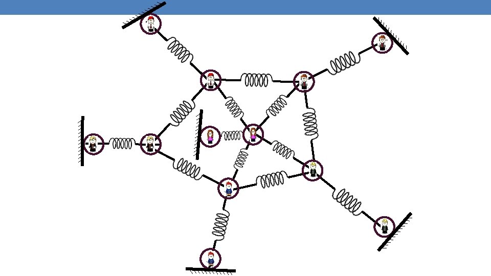
Springs and random walks • Our graph corresponds to an spring system • The Red node is pinned at position +1, while the Blue node is pinned at position -1 on a line. • There are springs on the edges with hardness proportional to the weights • The computed values are the positions of the nodes on the line
Springs and random walks • Our graph corresponds to an spring system • The Red node is pinned at position +1, while the Blue node is pinned at position -1 on a line. • There are springs on the edges with hardness proportional to the weights • The computed values are the positions of the nodes on the line 0. 16 -0. 16 0. 05
Opinion formation model (Friedkin and Johnsen) •
Opinion formation as a game • Inconsistency cost: The cost for deviating from one’s intrinsic opinion Conflict cost: The cost for disagreeing with the opinions in one’s social network D. Bindel, J. Kleinberg, S. Oren. How Bad is Forming Your Own Opinion? Proc. 52 nd IEEE Symposium on Foundations of Computer Science, 2011.
Opinion formation as a game • The Friedkin & Johnsen model
Example • Social network with internal opinions s = +0. 5 2 1 s = +0. 8 2 1 1 s = +0. 2 s = -0. 3 1 2 s = -0. 1 • There is a connection of this model with absorbing random walks and value propagation – can you see it?
Opinion formation and absorbing random walks s = +0. 5 Add to the network one absorbing node per user with value the intrinsic opinion of the user z = +0. 17 2 1 s = +0. 8 The expressed opinion for each node is computed using the value propagation we described • Repeated averaging 2 1 z = +0. 22 1 1 2 1 z = -0. 03 1 s = -0. 5 It is equal to the expected intrinsic opinion at the place of absorption s = -0. 3 z = -0. 01 z = 0. 04 1 s = -0. 1
Opinion of a user • For an individual user u • u’s absorbing node is a stationary point • u’s transient node is connected to the absorbing node with a spring. • The neighbors of u pull with their own springs.
Hitting time • A related quantity: Hitting time H(u, v) • The expected number of steps for a random walk starting from node u to end up in v for the first time • Make node v absorbing and compute the expected number of steps to reach v • Assumes that the graph is strongly connected, and there are no other absorbing nodes. • Commute time H(u, v) + H(v, u): often used as a distance metric • Proportional to the total resistance between nodes u, and v
Transductive learning • If we have a graph of relationships and some labels on some nodes we can propagate them to the remaining nodes • Make the labeled nodes to be absorbing and compute the probability for the rest of the graph • E. g. , a social network where some people are tagged as spammers • E. g. , the movie-actor graph where some movies are tagged as action or comedy. • This is a form of semi-supervised learning • We make use of the unlabeled data, and the relationships • It is also called transductive learning because it does not produce a model, but just labels the unlabeled data that is at hand. • Contrast to inductive learning that learns a model and can label any new example
Implementation details •