DATA MINING LECTURE 8 Sequence Segmentation Dimensionality Reduction

DATA MINING LECTURE 8 Sequence Segmentation Dimensionality Reduction

SEQUENCE SEGMENTATION

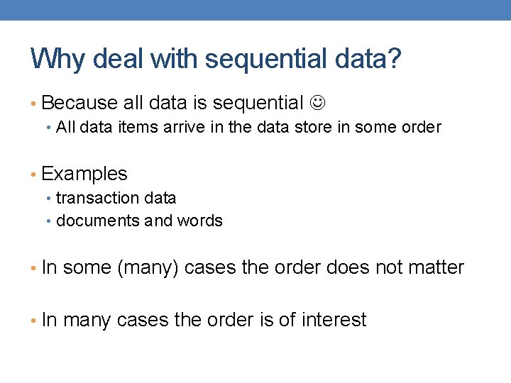
Why deal with sequential data? • Because all data is sequential • All data items arrive in the data store in some order • Examples • transaction data • documents and words • In some (many) cases the order does not matter • In many cases the order is of interest

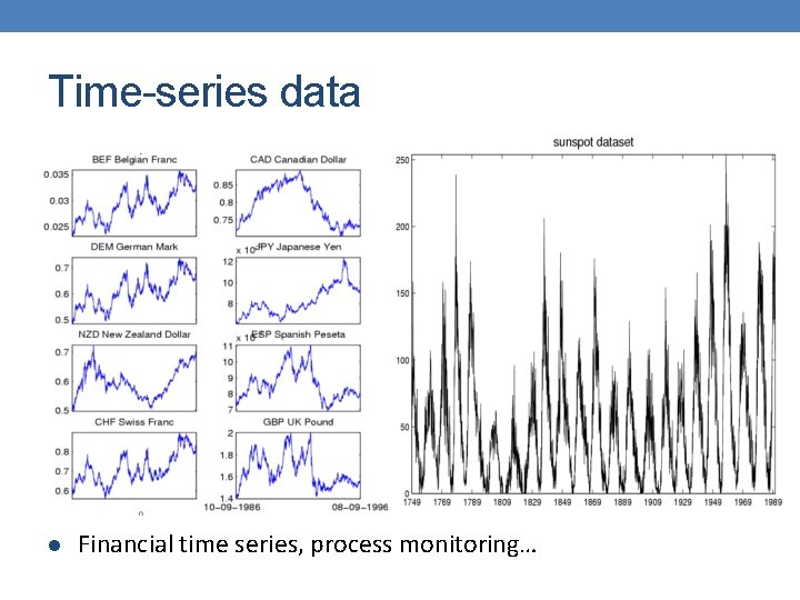
Time-series data l Financial time series, process monitoring…

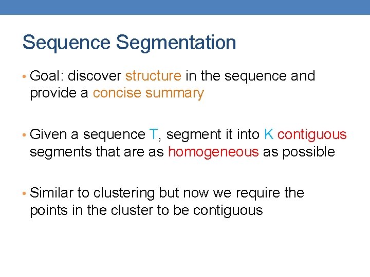
Sequence Segmentation • Goal: discover structure in the sequence and provide a concise summary • Given a sequence T, segment it into K contiguous segments that are as homogeneous as possible • Similar to clustering but now we require the points in the cluster to be contiguous

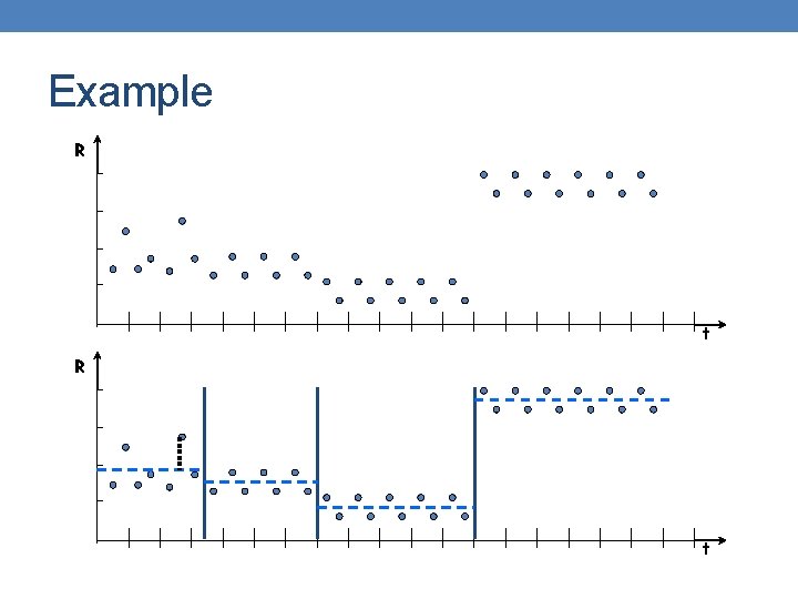
Example R t

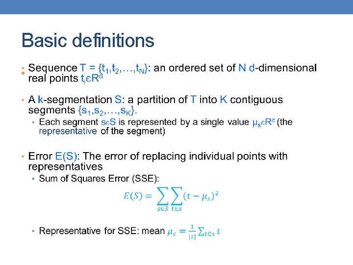
Basic definitions •

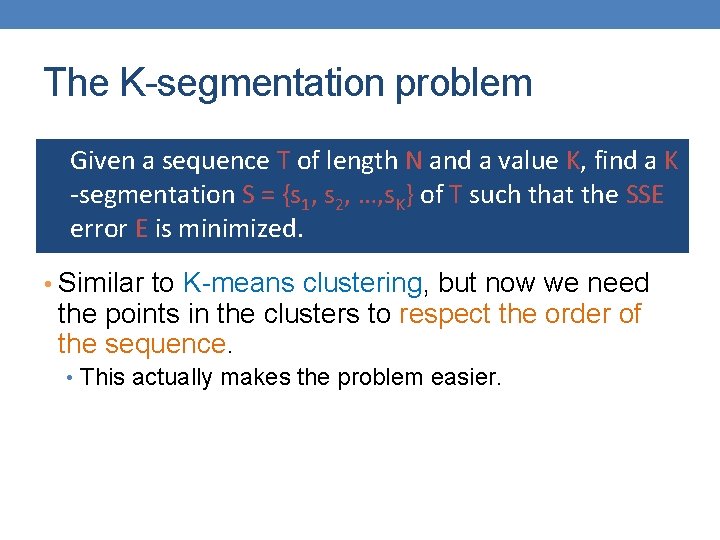
The K-segmentation problem l Given a sequence T of length N and a value K, find a K -segmentation S = {s 1, s 2, …, s. K} of T such that the SSE error E is minimized. • Similar to K-means clustering, but now we need the points in the clusters to respect the order of the sequence. • This actually makes the problem easier.

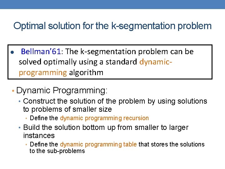
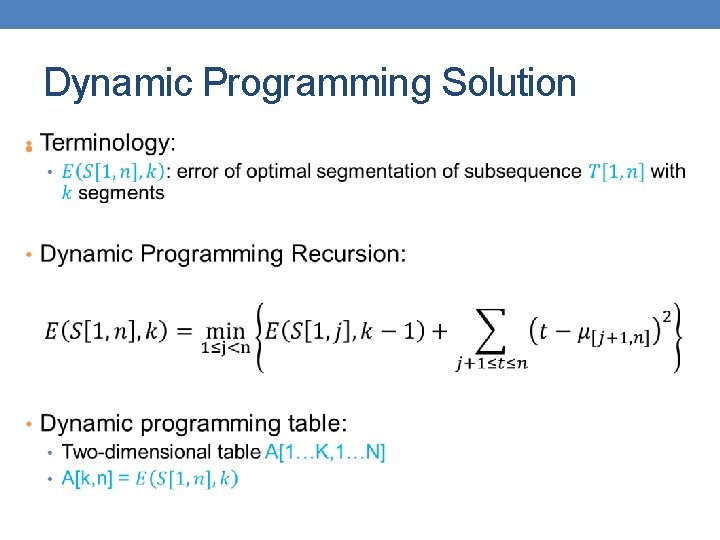
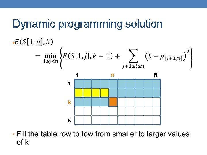
Optimal solution for the k-segmentation problem l [Bellman’ 61: The k-segmentation problem can be solved optimally using a standard dynamicprogramming algorithm • Dynamic Programming: • Construct the solution of the problem by using solutions to problems of smaller size • Define the dynamic programming recursion • Build the solution bottom up from smaller to larger instances • Define the dynamic programming table that stores the solutions to the sub-problems

Dynamic Programming Solution •

Dynamic programming solution • 1 1 k K n N

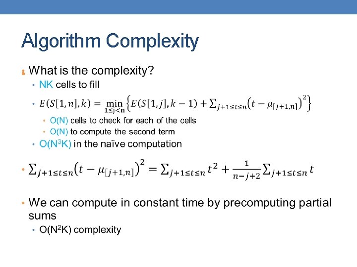
Algorithm Complexity •

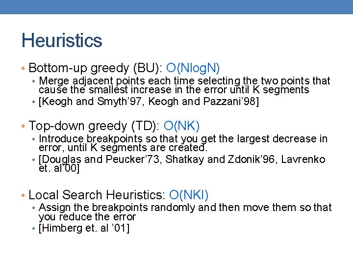
Heuristics • Bottom-up greedy (BU): O(Nlog. N) • Merge adjacent points each time selecting the two points that cause the smallest increase in the error until K segments • [Keogh and Smyth’ 97, Keogh and Pazzani’ 98] • Top-down greedy (TD): O(NK) • Introduce breakpoints so that you get the largest decrease in error, until K segments are created. • [Douglas and Peucker’ 73, Shatkay and Zdonik’ 96, Lavrenko et. al’ 00] • Local Search Heuristics: O(NKI) • Assign the breakpoints randomly and then move them so that you reduce the error • [Himberg et. al ’ 01]

DIMENSIONALITY REDUCTION

The curse of dimensionality • Real data usually have thousands, or millions of dimensions • E. g. , web documents, where the dimensionality is the vocabulary of words • Facebook graph, where the dimensionality is the number of users • Huge number of dimensions causes many problems • Data becomes very sparse, some algorithms become meaningless (e. g. density based clustering) • The complexity of several algorithms depends on the dimensionality and they become infeasible.

Dimensionality Reduction • Usually the data can be described with fewer dimensions, without losing much of the meaning of the data. • The data reside in a space of lower dimensionality • Essentially, we assume that some of the data is noise, and we can approximate the useful part with a lower dimensionality space. • Dimensionality reduction does not just reduce the amount of data, it often brings out the useful part of the data

Data in the form of a matrix • We are given n objects and d attributes describing the objects. Each object has d numeric values describing it. • We will represent the data as a n d real matrix A. • We can now use tools from linear algebra to process the data matrix • Our goal is to produce a new n k matrix B such that • It preserves as much of the information in the original matrix A as possible • It reveals something about the structure of the data in A

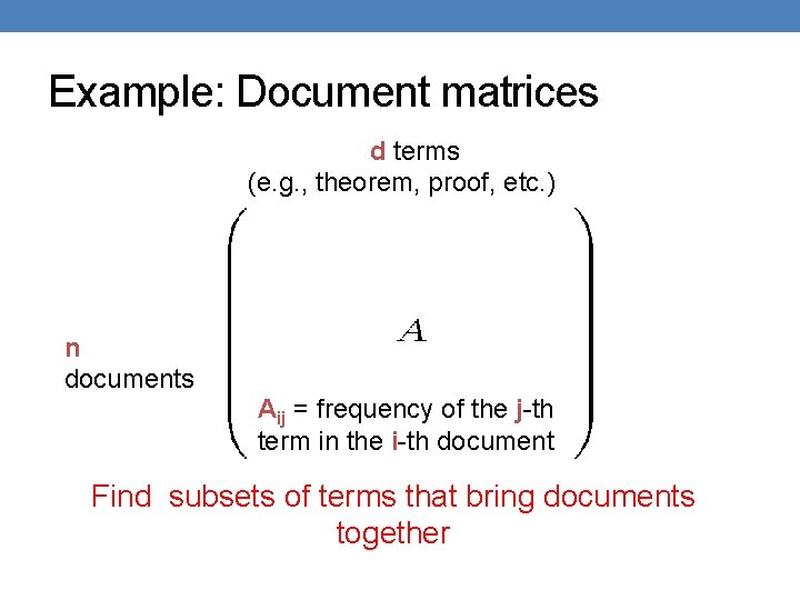
Example: Document matrices d terms (e. g. , theorem, proof, etc. ) n documents Aij = frequency of the j-th term in the i-th document Find subsets of terms that bring documents together

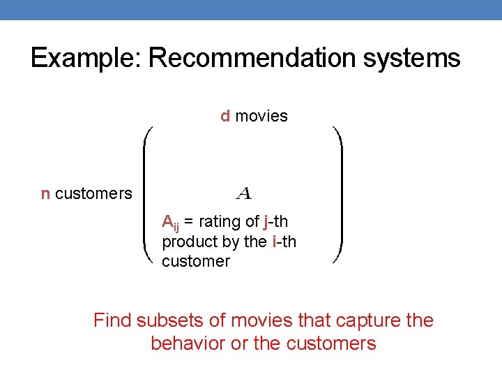
Example: Recommendation systems d movies n customers Aij = rating of j-th product by the i-th customer Find subsets of movies that capture the behavior or the customers

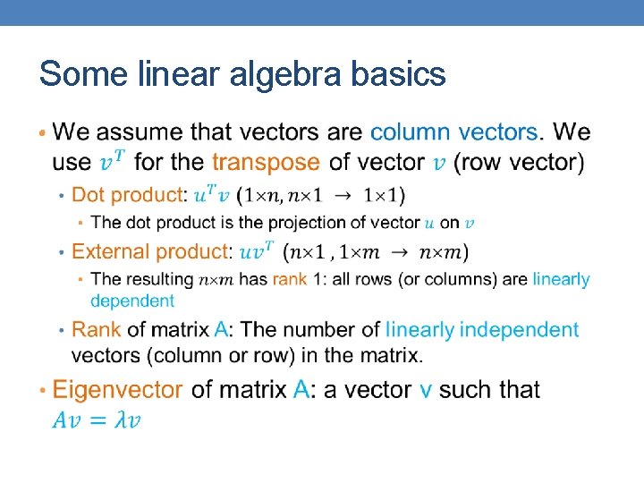
Some linear algebra basics •

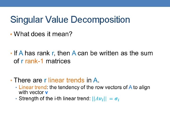
Singular Value Decomposition [n×r] [r×n] • r : rank of matrix A • σ1≥ σ2≥ … ≥σr : singular values (square roots of eig-vals AAT, ATA) • • • : left singular vectors (eig-vectors of AAT) : right singular vectors (eig-vectors of ATA)

Singular Value Decomposition •

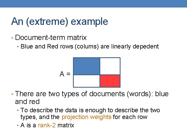
An (extreme) example • Document-term matrix • Blue and Red rows (colums) are linearly depedent A= • There are two types of documents (words): blue and red • To describe the data is enough to describe the two types, and the projection weights for each row • A is a rank-2 matrix

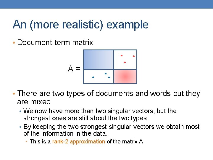
An (more realistic) example • Document-term matrix A= • There are two types of documents and words but they are mixed • We now have more than two singular vectors, but the strongest ones are still about the two types. • By keeping the two strongest singular vectors we obtain most of the information in the data. • This is a rank-2 approximation of the matrix A

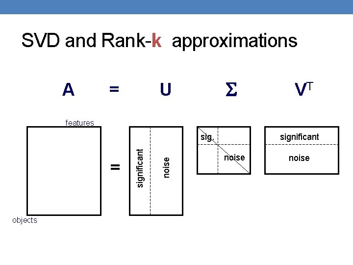
SVD and Rank-k approximations A = U VT features objects noise = significant noise

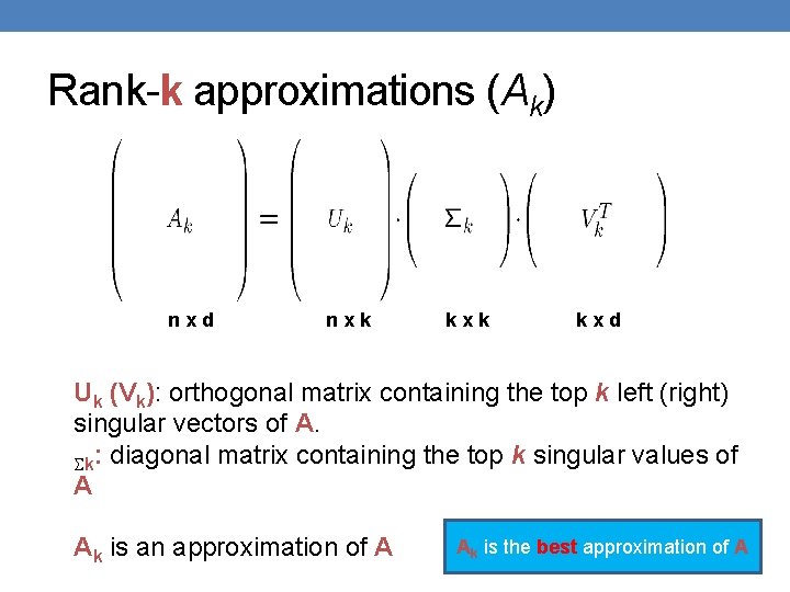
Rank-k approximations (Ak) nxd nxk kxd Uk (Vk): orthogonal matrix containing the top k left (right) singular vectors of A. Sk: diagonal matrix containing the top k singular values of A Ak is an approximation of A Ak is the best approximation of A

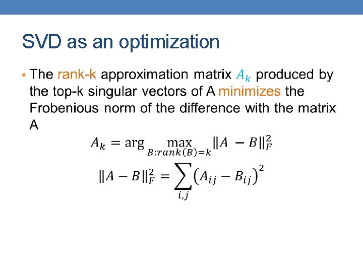
SVD as an optimization •

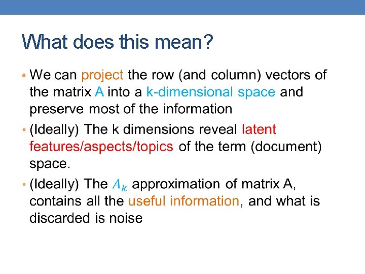
What does this mean? •

Two applications • Latent Semantic Indexing (LSI): • Apply SVD on the document-term space, and index the kdimensional vectors • When a query comes, project it onto the low dimensional space and compute similarity cosine similarity in this space • Singular vectors capture main topics, and enrich the document representation • Recommender systems and collaborative filtering • In a movie-rating system there are just a few types of users. • What we observe is an incomplete and noisy version of the true data • The rank-k approximation reconstructs the “true” matrix and we can provide ratings for movies that are not rated.

SVD and PCA • PCA is a special case of SVD on the centered covariance matrix.

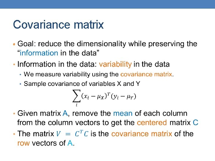
Covariance matrix •

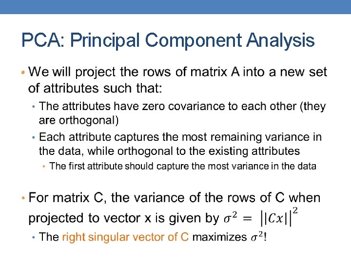
PCA: Principal Component Analysis •

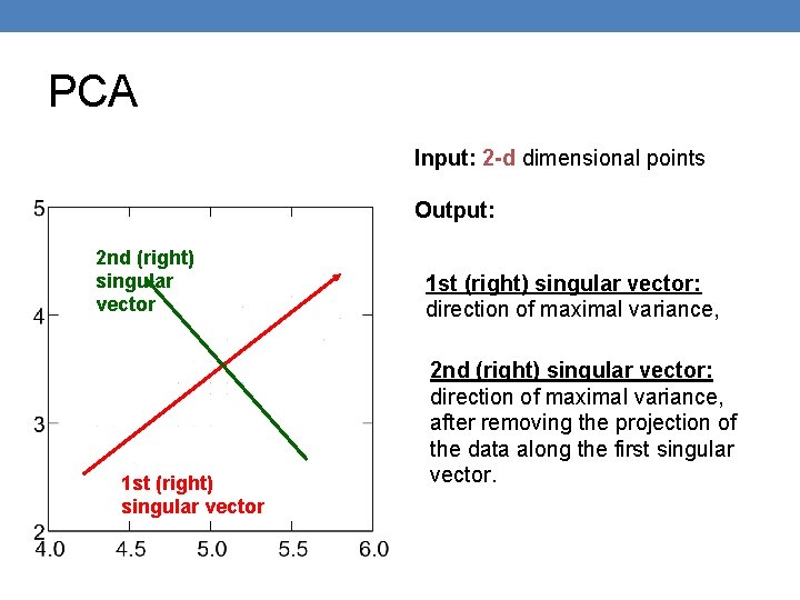
PCA Input: 2 -d dimensional points Output: 2 nd (right) singular vector 1 st (right) singular vector: direction of maximal variance, 2 nd (right) singular vector: direction of maximal variance, after removing the projection of the data along the first singular vector.

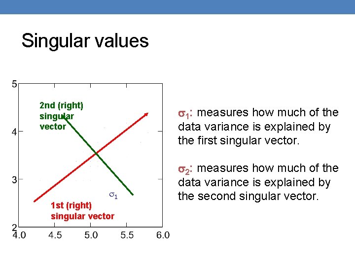
Singular values 2 nd (right) singular vector 1: measures how much of the data variance is explained by the first singular vector. 1 1 st (right) singular vector 2: measures how much of the data variance is explained by the second singular vector.

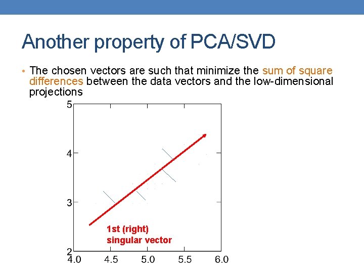
Another property of PCA/SVD • The chosen vectors are such that minimize the sum of square differences between the data vectors and the low-dimensional projections 1 st (right) singular vector

SVD is “the Rolls-Royce and the Swiss Army Knife of Numerical Linear Algebra. ”* *Dianne O’Leary, MMDS ’ 06