DATA MINING LECTURE 7 Hierarchical Clustering DBSCAN The
DATA MINING LECTURE 7 Hierarchical Clustering, DBSCAN The EM Algorithm

CLUSTERING
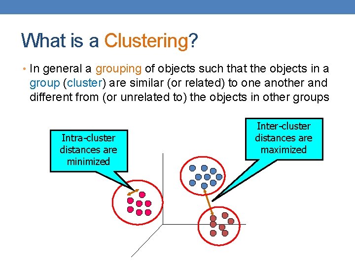
What is a Clustering? • In general a grouping of objects such that the objects in a group (cluster) are similar (or related) to one another and different from (or unrelated to) the objects in other groups Intra-cluster distances are minimized Inter-cluster distances are maximized
Clustering Algorithms • K-means and its variants • Hierarchical clustering • DBSCAN

HIERARCHICAL CLUSTERING
Hierarchical Clustering • Two main types of hierarchical clustering • Agglomerative: • Start with the points as individual clusters • At each step, merge the closest pair of clusters until only one cluster (or k clusters) left • Divisive: • Start with one, all-inclusive cluster • At each step, split a cluster until each cluster contains a point (or there are k clusters) • Traditional hierarchical algorithms use a similarity or distance matrix • Merge or split one cluster at a time
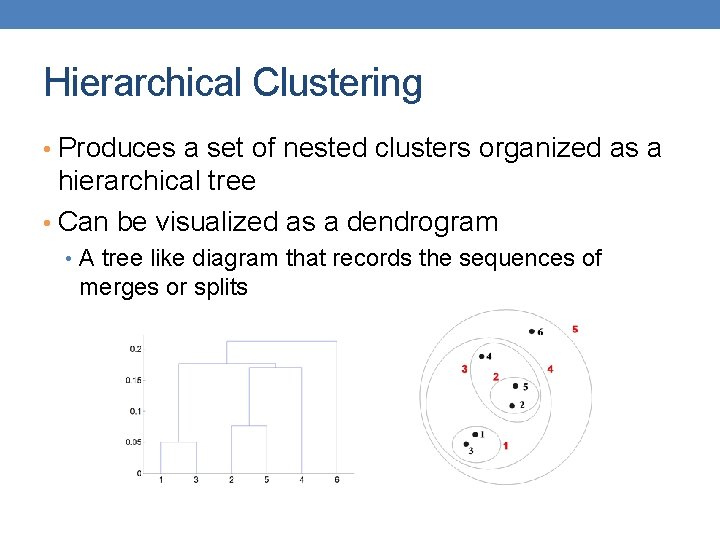
Hierarchical Clustering • Produces a set of nested clusters organized as a hierarchical tree • Can be visualized as a dendrogram • A tree like diagram that records the sequences of merges or splits
Strengths of Hierarchical Clustering • Do not have to assume any particular number of clusters • Any desired number of clusters can be obtained by ‘cutting’ the dendogram at the proper level • They may correspond to meaningful taxonomies • Example in biological sciences (e. g. , animal kingdom, phylogeny reconstruction, …)
Agglomerative Clustering Algorithm • More popular hierarchical clustering technique • Basic algorithm is straightforward 1. 2. 3. 4. 5. 6. • Compute the proximity matrix Let each data point be a cluster Repeat Merge the two closest clusters Update the proximity matrix Until only a single cluster remains Key operation is the computation of the proximity of two clusters • Different approaches to defining the distance between clusters distinguish the different algorithms
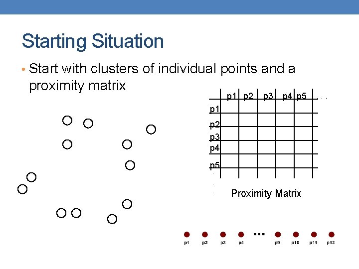
Starting Situation • Start with clusters of individual points and a proximity matrix p 1 p 2 p 3 p 4 p 5. . . Proximity Matrix . . .
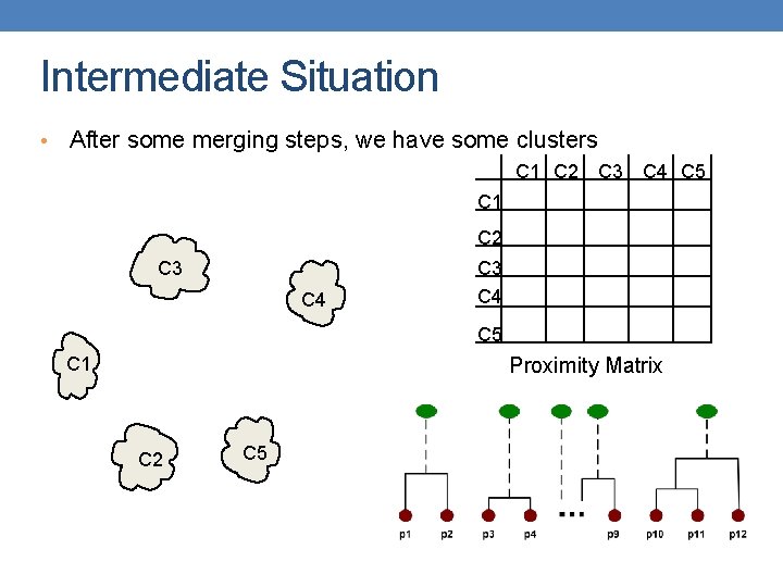
Intermediate Situation • After some merging steps, we have some clusters C 1 C 2 C 3 C 4 C 5 C 1 Proximity Matrix C 2 C 5
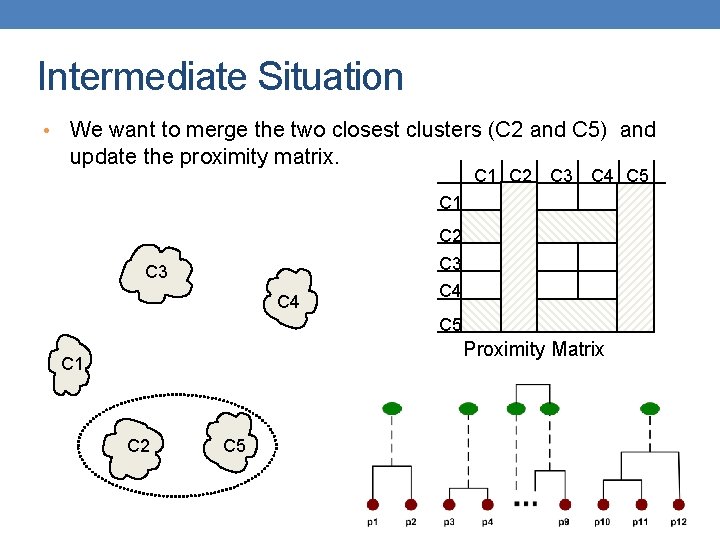
Intermediate Situation • We want to merge the two closest clusters (C 2 and C 5) and update the proximity matrix. C 1 C 2 C 3 C 4 C 5 Proximity Matrix C 1 C 2 C 5
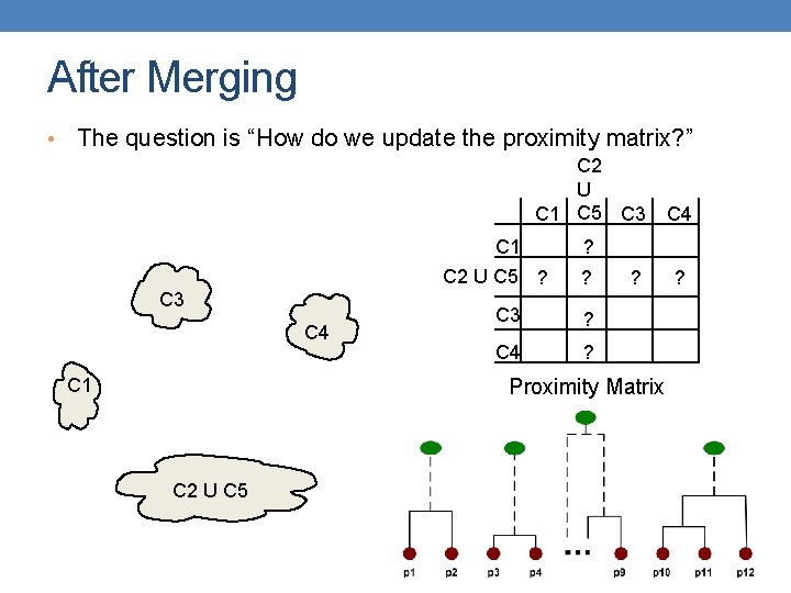
After Merging • The question is “How do we update the proximity matrix? ” C 2 U C 1 C 5 C 3 C 1 C 2 U C 5 ? C 3 C 4 C 1 ? ? C 3 ? C 4 ? ? Proximity Matrix C 2 U C 5 C 4 ?
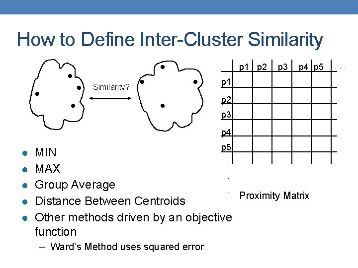
How to Define Inter-Cluster Similarity p 1 p 2 Similarity? p 3 p 4 p 5 p 1 p 2 p 3 p 4 l l l p 5 MIN. MAX. Group Average. Proximity Matrix Distance Between Centroids Other methods driven by an objective function – Ward’s Method uses squared error . . .
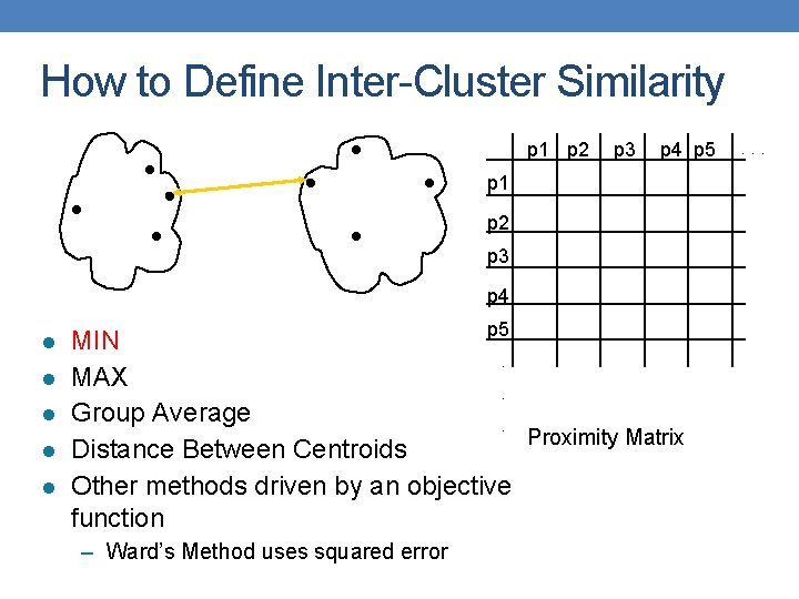
How to Define Inter-Cluster Similarity p 1 p 2 p 3 p 4 p 5 p 1 p 2 p 3 p 4 l l l p 5 MIN. MAX. Group Average. Proximity Matrix Distance Between Centroids Other methods driven by an objective function – Ward’s Method uses squared error . . .
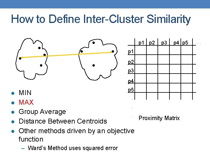
How to Define Inter-Cluster Similarity p 1 p 2 p 3 p 4 p 5 p 1 p 2 p 3 p 4 l l l p 5 MIN. MAX. Group Average. Proximity Matrix Distance Between Centroids Other methods driven by an objective function – Ward’s Method uses squared error . . .
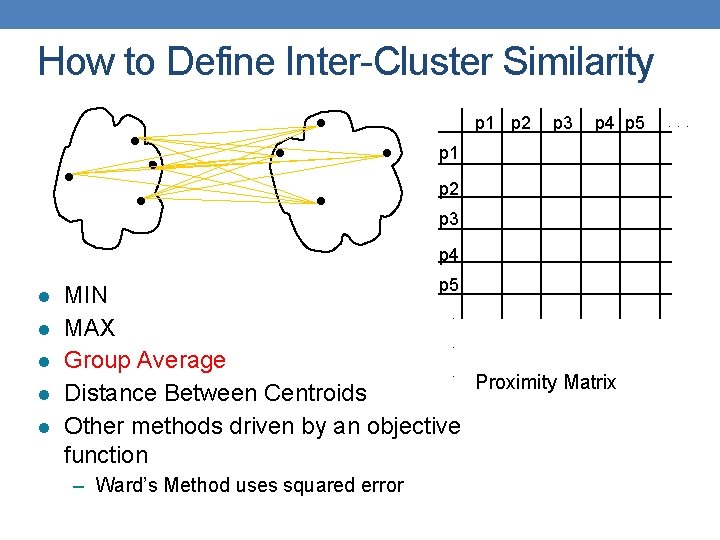
How to Define Inter-Cluster Similarity p 1 p 2 p 3 p 4 p 5 p 1 p 2 p 3 p 4 l l l p 5 MIN. MAX. Group Average. Proximity Matrix Distance Between Centroids Other methods driven by an objective function – Ward’s Method uses squared error . . .
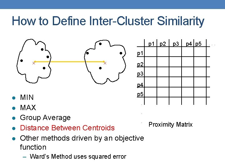
How to Define Inter-Cluster Similarity p 1 p 2 p 3 p 4 p 5 p 1 p 2 p 3 p 4 l l l p 5 MIN. MAX. Group Average. Proximity Matrix Distance Between Centroids Other methods driven by an objective function – Ward’s Method uses squared error . . .
Single Link – Complete Link • Another way to view the processing of the hierarchical algorithm is that we create links between their elements in order of increasing distance • The MIN – Single Link, will merge two clusters when a single pair of elements is linked • The MAX – Complete Linkage will merge two clusters when all pairs of elements have been linked.
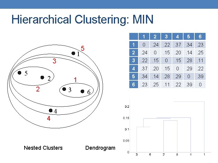
Hierarchical Clustering: MIN 1 1 3 5 2 1 2 3 4 5 6 4 Nested Clusters Dendrogram 2 3 4 5 1 0 2 . 24 3 . 22. 15 4 . 37. 20. 15 5 . 34. 14. 28. 29 6 . 23. 25. 11. 22. 39 6 . 24. 22. 37. 34. 23 0 . 15. 20. 14. 25 0 . 15. 28. 11 0 . 29. 22 0 . 39 0
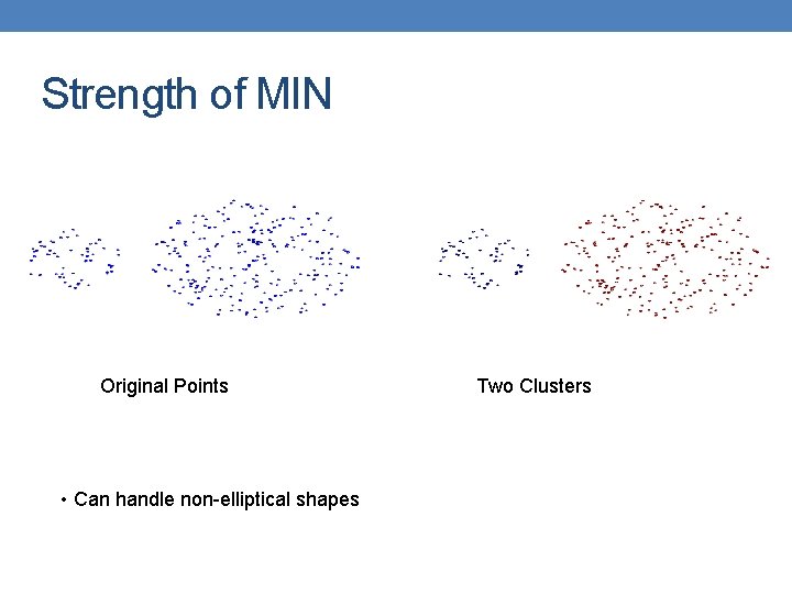
Strength of MIN Original Points • Can handle non-elliptical shapes Two Clusters
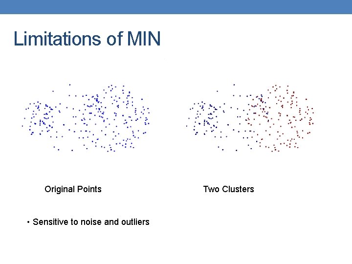
Limitations of MIN Original Points • Sensitive to noise and outliers Two Clusters
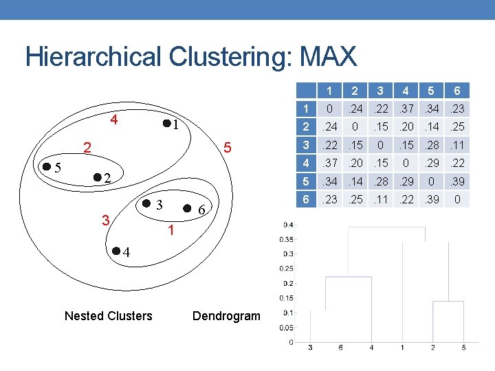
Hierarchical Clustering: MAX 1 4 1 5 2 3 3 6 1 4 Nested Clusters Dendrogram 2 3 4 5 1 0 2 . 24 3 . 22. 15 4 . 37. 20. 15 5 . 34. 14. 28. 29 6 . 23. 25. 11. 22. 39 6 . 24. 22. 37. 34. 23 0 . 15. 20. 14. 25 0 . 15. 28. 11 0 . 29. 22 0 . 39 0
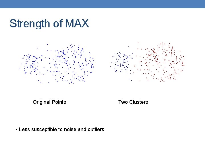
Strength of MAX Original Points • Less susceptible to noise and outliers Two Clusters
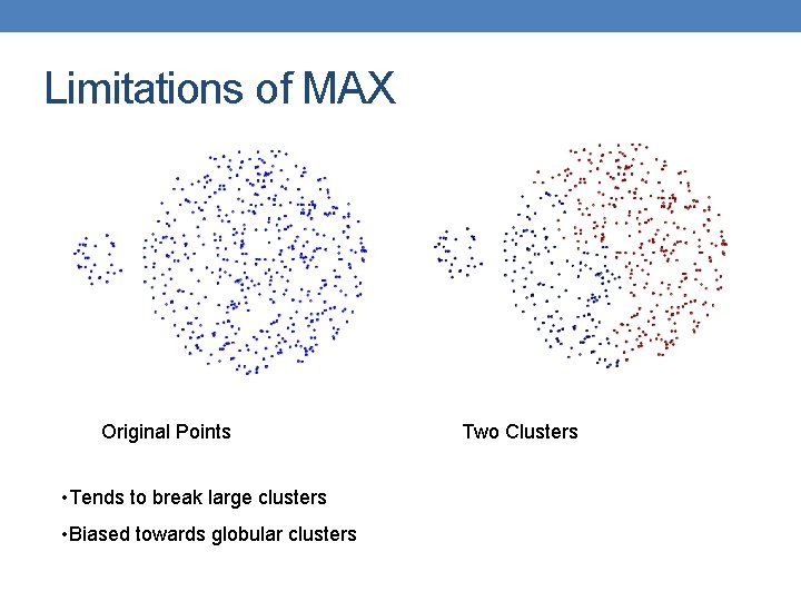
Limitations of MAX Original Points • Tends to break large clusters • Biased towards globular clusters Two Clusters
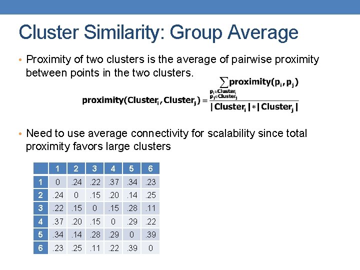
Cluster Similarity: Group Average • Proximity of two clusters is the average of pairwise proximity between points in the two clusters. • Need to use average connectivity for scalability since total proximity favors large clusters 1 2 3 4 5 1 0 2 . 24 3 . 22. 15 4 . 37. 20. 15 5 . 34. 14. 28. 29 6 . 23. 25. 11. 22. 39 6 . 24. 22. 37. 34. 23 0 . 15. 20. 14. 25 0 . 15. 28. 11 0 . 29. 22 0 . 39 0
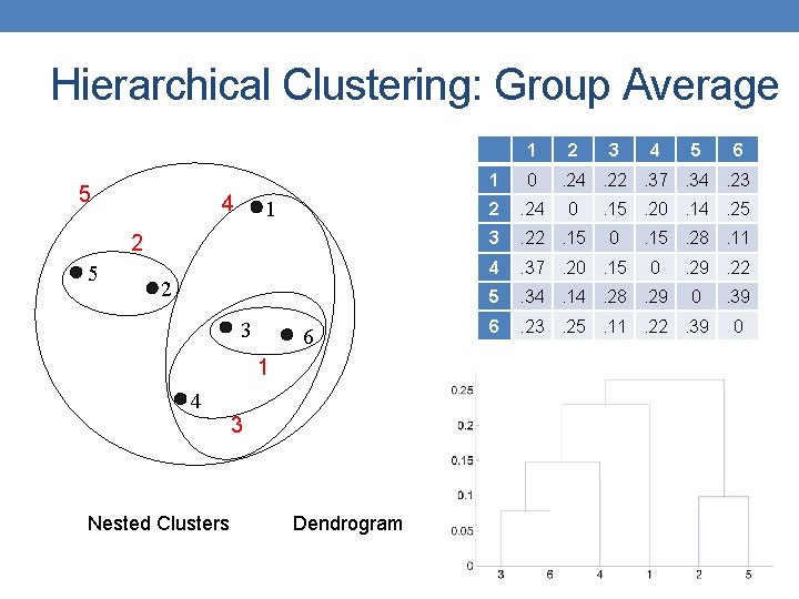
Hierarchical Clustering: Group Average 1 5 4 1 2 5 2 3 6 1 4 Nested Clusters 3 Dendrogram 2 3 4 5 1 0 2 . 24 3 . 22. 15 4 . 37. 20. 15 5 . 34. 14. 28. 29 6 . 23. 25. 11. 22. 39 6 . 24. 22. 37. 34. 23 0 . 15. 20. 14. 25 0 . 15. 28. 11 0 . 29. 22 0 . 39 0
Hierarchical Clustering: Group Average • Compromise between Single and Complete Link • Strengths • • Less susceptible to noise and outliers Limitations • Biased towards globular clusters
Cluster Similarity: Ward’s Method • Similarity of two clusters is based on the increase in squared error (SSE) when two clusters are merged • Similar to group average if distance between points is distance squared • Less susceptible to noise and outliers • Biased towards globular clusters • Hierarchical analogue of K-means • Can be used to initialize K-means
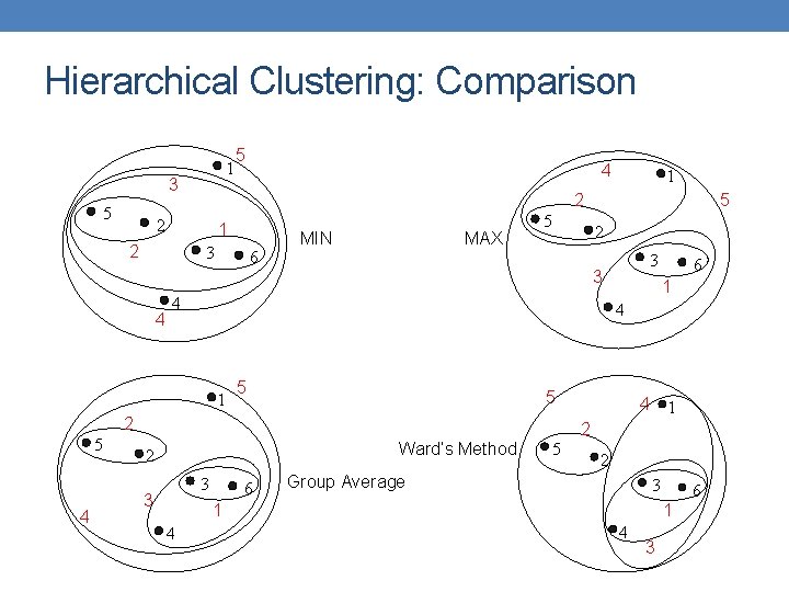
Hierarchical Clustering: Comparison 1 3 5 5 1 2 3 6 MIN MAX 5 2 5 1 5 Ward’s Method 3 6 4 1 2 5 2 Group Average 3 1 4 6 4 2 3 3 3 2 4 5 4 1 5 1 2 2 4 4 6 1 4 3
Hierarchical Clustering: Time and Space requirements • O(N 2) space since it uses the proximity matrix. • N is the number of points. • O(N 3) time in many cases • There are N steps and at each step the size, N 2, proximity matrix must be updated and searched • Complexity can be reduced to O(N 2 log(N) ) time for some approaches
Hierarchical Clustering: Problems and Limitations • Computational complexity in time and space • Once a decision is made to combine two clusters, it cannot be undone • No objective function is directly minimized • Different schemes have problems with one or more of the following: • Sensitivity to noise and outliers • Difficulty handling different sized clusters and convex shapes • Breaking large clusters

DBSCAN
DBSCAN: Density-Based Clustering • DBSCAN is a Density-Based Clustering algorithm • Reminder: In density based clustering we partition points into dense regions separated by not-so-dense regions. • Important Questions: • How do we measure density? • What is a dense region? • DBSCAN: • Density at point p: number of points within a circle of radius Eps • Dense Region: A circle of radius Eps that contains at least Min. Pts points
DBSCAN • Characterization of points • A point is a core point if it has more than a specified number of points (Min. Pts) within Eps • These points belong in a dense region and are at the interior of a cluster • A border point has fewer than Min. Pts within Eps, but is in the neighborhood of a core point. • A noise point is any point that is not a core point or a border point.
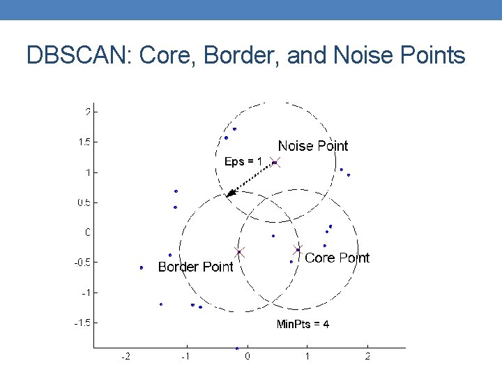
DBSCAN: Core, Border, and Noise Points
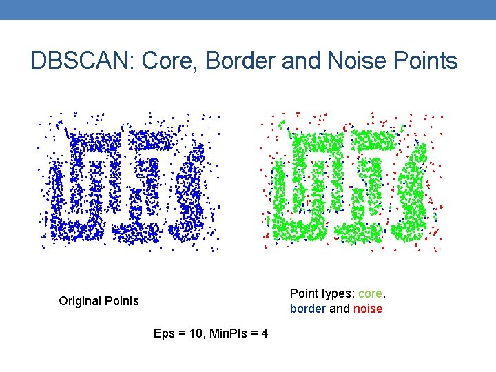
DBSCAN: Core, Border and Noise Points Point types: core, border and noise Original Points Eps = 10, Min. Pts = 4
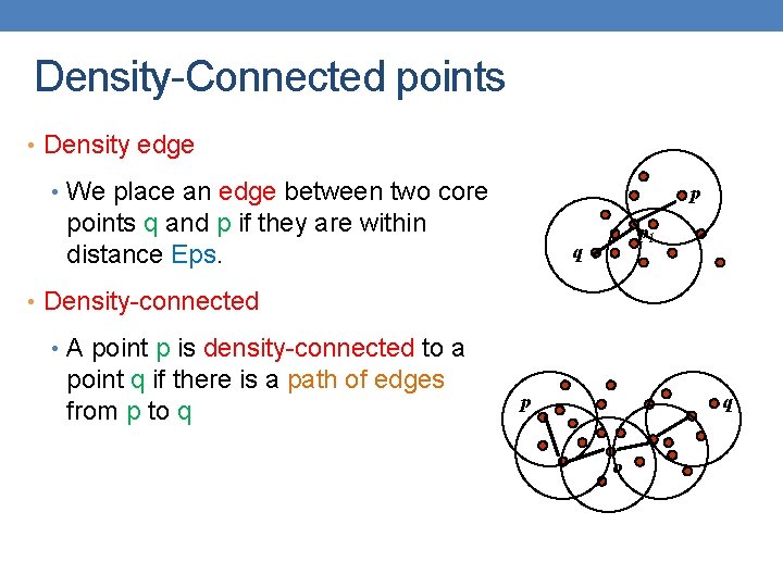
Density-Connected points • Density edge • We place an edge between two core p points q and p if they are within distance Eps. p 1 q • Density-connected • A point p is density-connected to a point q if there is a path of edges from p to q p q o
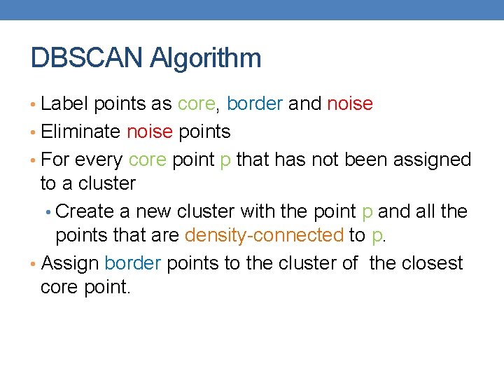
DBSCAN Algorithm • Label points as core, border and noise • Eliminate noise points • For every core point p that has not been assigned to a cluster • Create a new cluster with the point p and all the points that are density-connected to p. • Assign border points to the cluster of the closest core point.
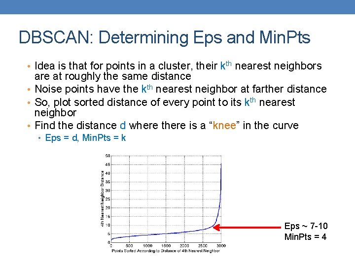
DBSCAN: Determining Eps and Min. Pts • Idea is that for points in a cluster, their kth nearest neighbors are at roughly the same distance • Noise points have the kth nearest neighbor at farther distance • So, plot sorted distance of every point to its kth nearest neighbor • Find the distance d where there is a “knee” in the curve • Eps = d, Min. Pts = k Eps ~ 7 -10 Min. Pts = 4
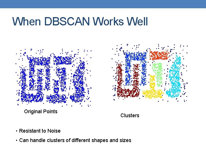
When DBSCAN Works Well Original Points Clusters • Resistant to Noise • Can handle clusters of different shapes and sizes
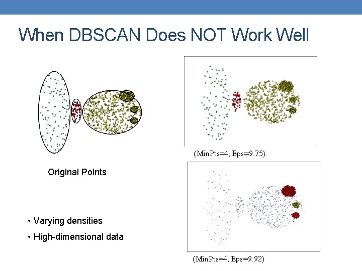
When DBSCAN Does NOT Work Well (Min. Pts=4, Eps=9. 75). Original Points • Varying densities • High-dimensional data (Min. Pts=4, Eps=9. 92)
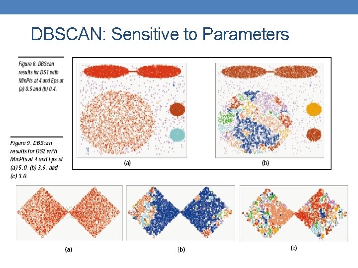
DBSCAN: Sensitive to Parameters
Other algorithms • PAM, CLARANS: Solutions for the k-medoids problem • BIRCH: Constructs a hierarchical tree that acts a summary of the data, and then clusters the leaves. • MST: Clustering using the Minimum Spanning Tree. • ROCK: clustering categorical data by neighbor and link analysis • LIMBO, COOLCAT: Clustering categorical data using information theoretic tools. • CURE: Hierarchical algorithm uses different representation of the cluster • CHAMELEON: Hierarchical algorithm uses closeness and interconnectivity for merging
MIXTURE MODELS AND THE EM ALGORITHM
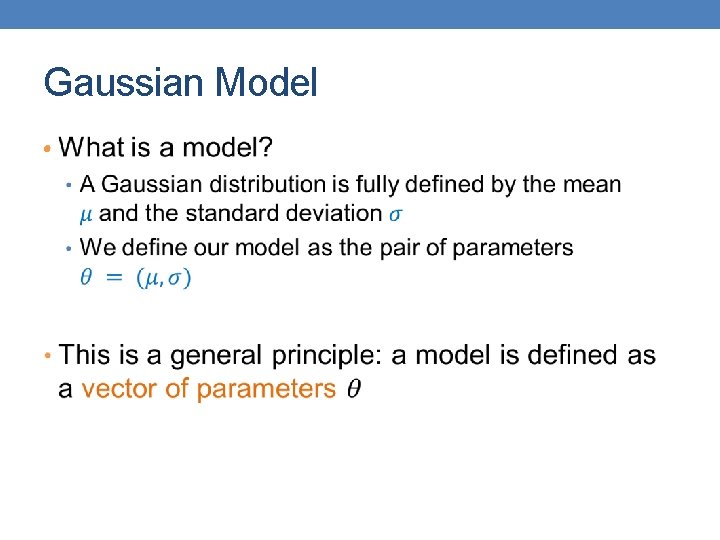
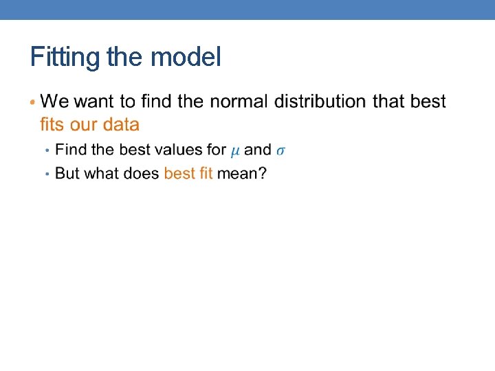
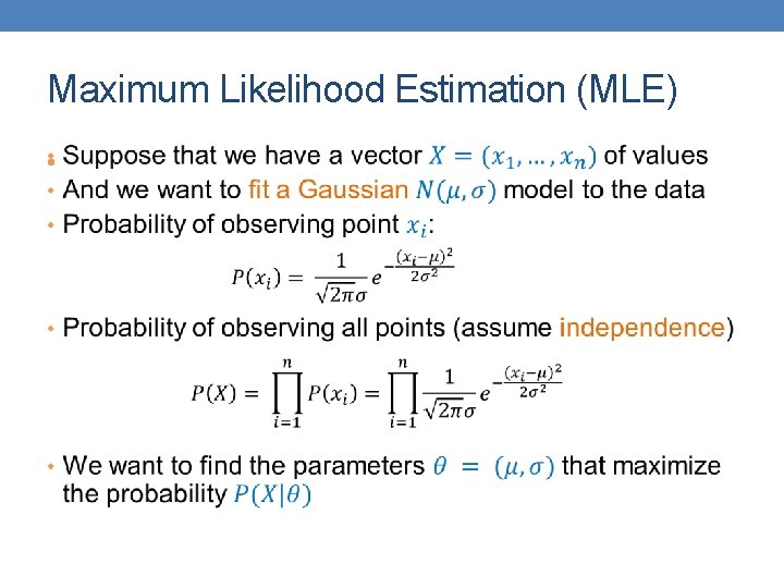
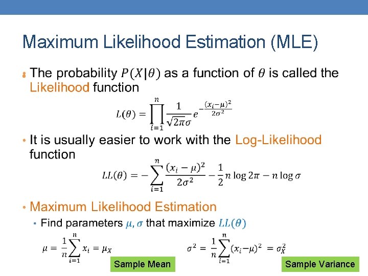
Model-based clustering • In order to understand our data, we will assume that there is a generative process (a model) that creates/describes the data, and we will try to find the model that best fits the data. • Models of different complexity can be defined, but we will assume that our model is a distribution from which data points are sampled • Example: the data is the height of all people in Greece • In most cases, a single distribution is not good enough to describe all data points: different parts of the data follow a different distribution • Example: the data is the height of all people in Greece and China • We need a mixture model • Different distributions correspond to different clusters in the data.
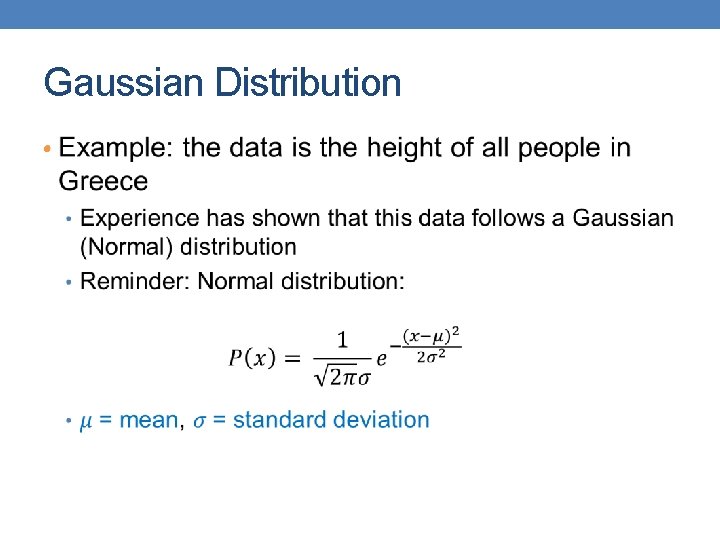
Gaussian Distribution •
Gaussian Model •
Fitting the model •
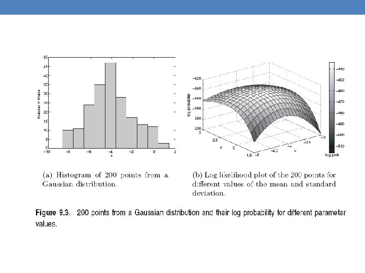
Maximum Likelihood Estimation (MLE) •
Maximum Likelihood Estimation (MLE) • Sample Mean Sample Variance
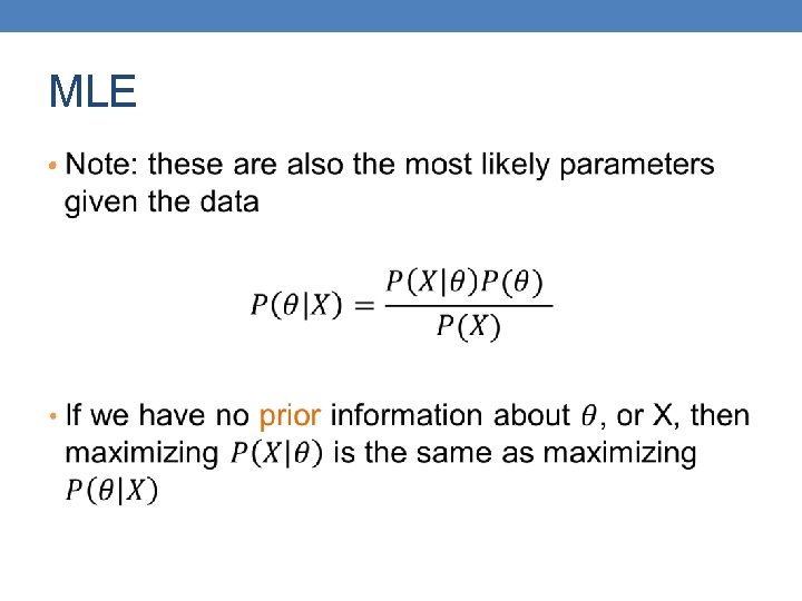
MLE •
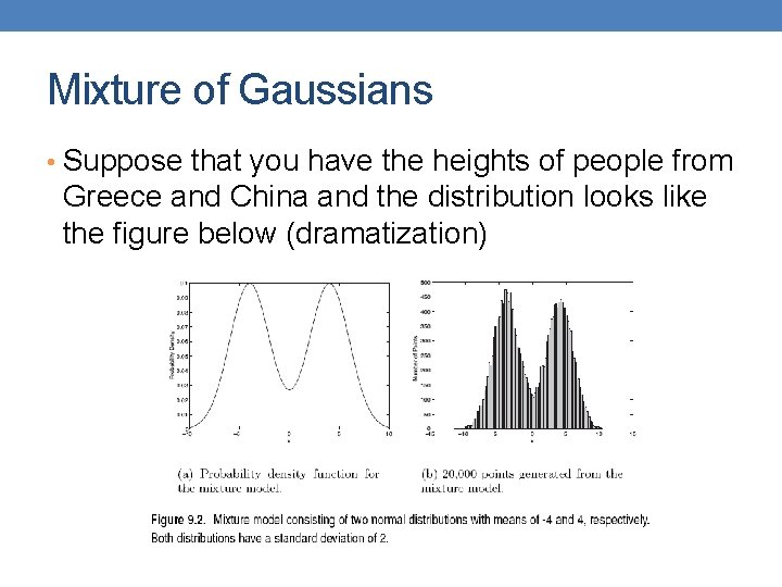
Mixture of Gaussians • Suppose that you have the heights of people from Greece and China and the distribution looks like the figure below (dramatization)
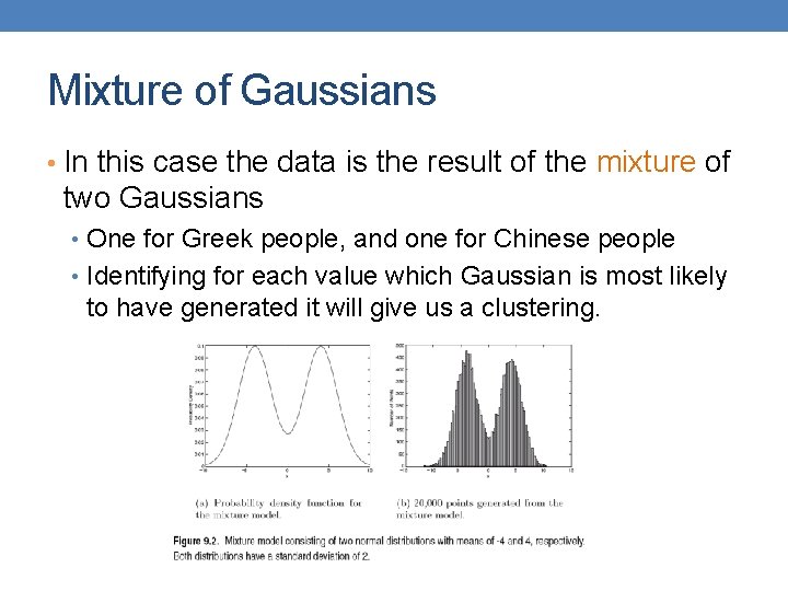
Mixture of Gaussians • In this case the data is the result of the mixture of two Gaussians • One for Greek people, and one for Chinese people • Identifying for each value which Gaussian is most likely to have generated it will give us a clustering.
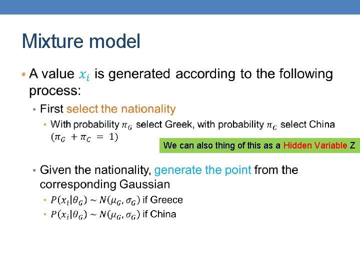
Mixture model • We can also thing of this as a Hidden Variable Z
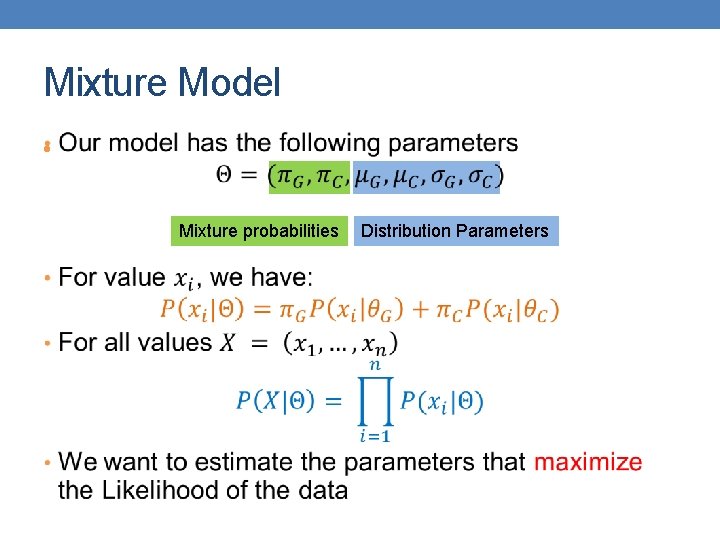
Mixture Model • Mixture probabilities Distribution Parameters
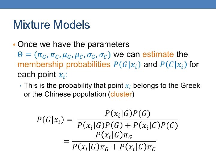
Mixture Models •
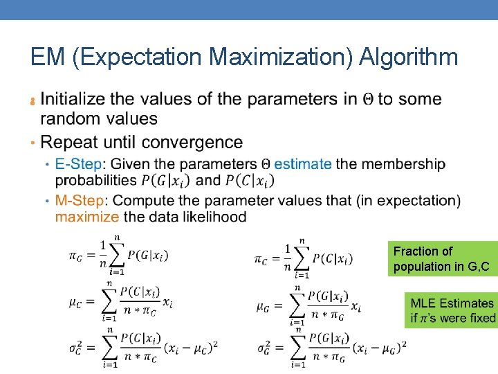
EM (Expectation Maximization) Algorithm • Fraction of population in G, C
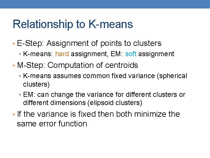
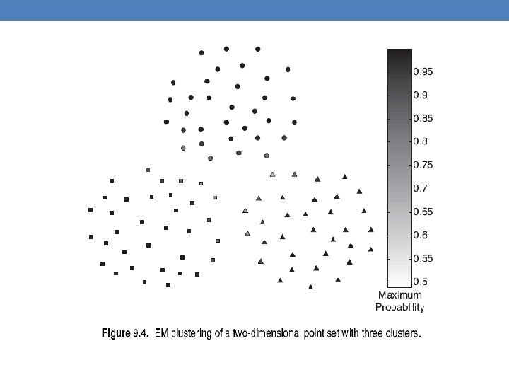
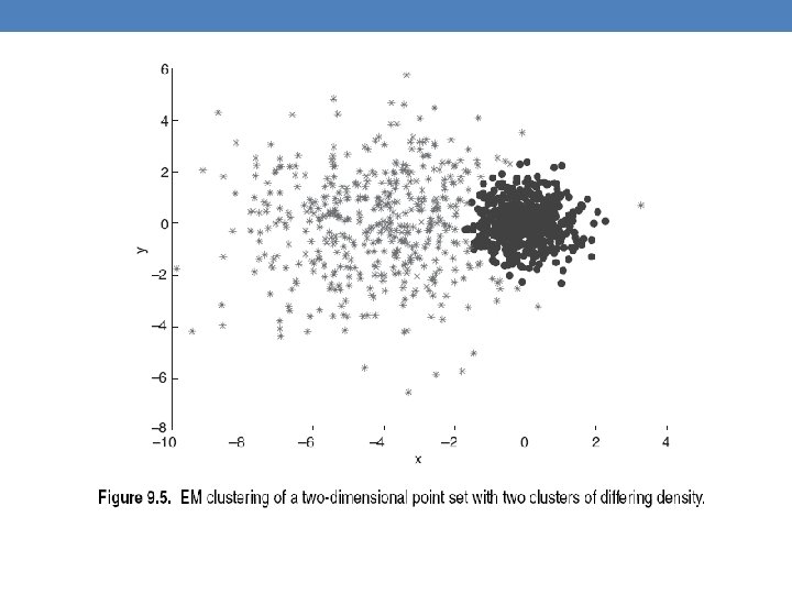
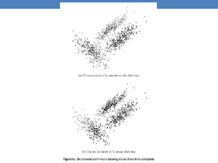
Relationship to K-means • E-Step: Assignment of points to clusters • K-means: hard assignment, EM: soft assignment • M-Step: Computation of centroids • K-means assumes common fixed variance (spherical clusters) • EM: can change the variance for different clusters or different dimensions (elipsoid clusters) • If the variance is fixed then both minimize the same error function
- Slides: 63