DATA MINING LECTURE 6 MinHashing Locality Sensitive Hashing

DATA MINING LECTURE 6 Min-Hashing, Locality Sensitive Hashing Clustering

MIN-HASHING AND LOCALITY SENSITIVE HASHING Thanks to: Rajaraman and Ullman, “Mining Massive Datasets” Evimaria Terzi, slides for Data Mining Course.

Motivating problem • Find duplicate and near-duplicate documents from a web crawl. • If we wanted exact duplicates we could do this by hashing • We will see how to adapt this technique for near duplicate documents

Main issues • What is the right representation of the document when we check for similarity? • E. g. , representing a document as a set of characters will not do (why? ) • When we have billions of documents, keeping the full text in memory is not an option. • We need to find a shorter representation • How do we do pairwise comparisons of billions of documents? • If exact match was the issue it would be ok, can we replicate this idea?

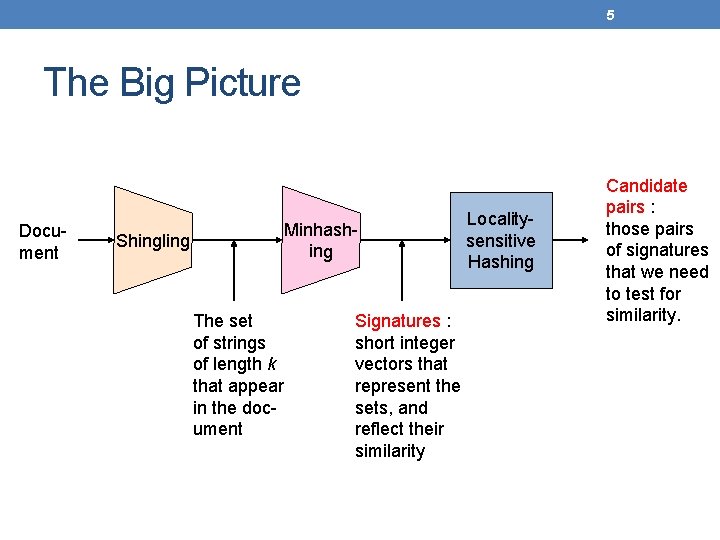
5 The Big Picture Document Shingling Minhashing The set of strings of length k that appear in the document Signatures : short integer vectors that represent the sets, and reflect their similarity Localitysensitive Hashing Candidate pairs : those pairs of signatures that we need to test for similarity.

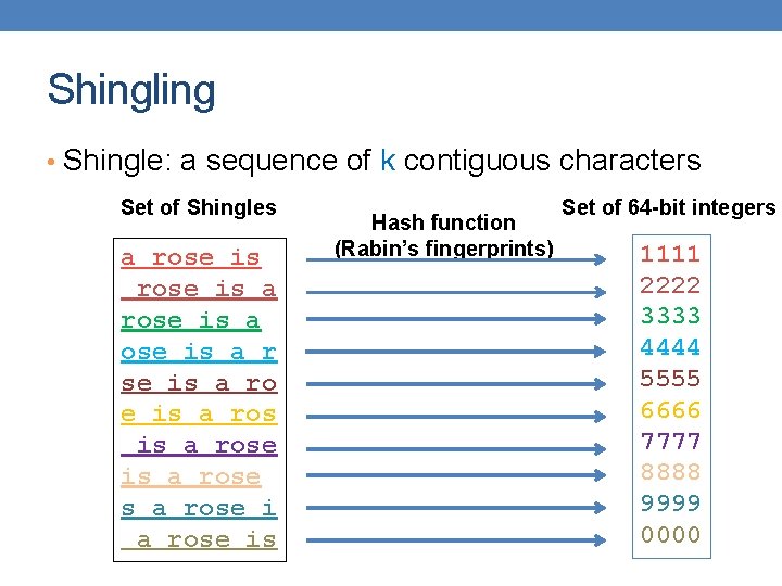
Shingling • Shingle: a sequence of k contiguous characters Set of Shingles a rose is a r se is a rose is a rose is Hash function (Rabin’s fingerprints) Set of 64 -bit integers 1111 2222 3333 4444 5555 6666 7777 8888 9999 0000

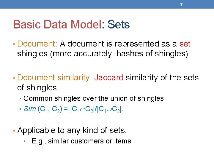
7 Basic Data Model: Sets • Document: A document is represented as a set shingles (more accurately, hashes of shingles) • Document similarity: Jaccard similarity of the sets of shingles. • Common shingles over the union of shingles • Sim (C 1, C 2) = |C 1 C 2|/|C 1 C 2|. • Applicable to any kind of sets. • E. g. , similar customers or items.

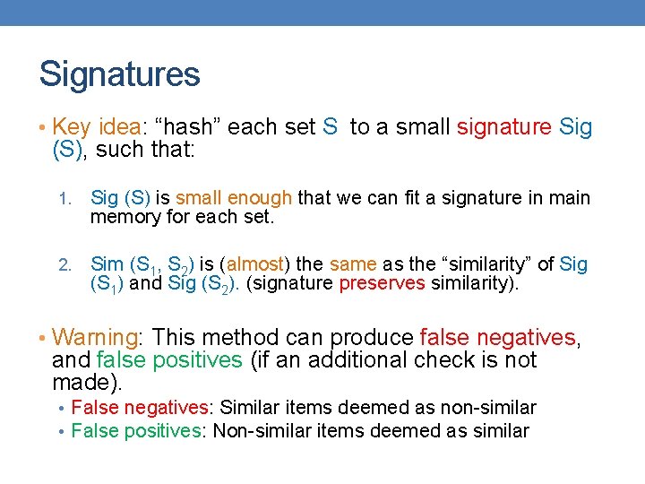
Signatures • Key idea: “hash” each set S to a small signature Sig (S), such that: 1. Sig (S) is small enough that we can fit a signature in main memory for each set. 2. Sim (S 1, S 2) is (almost) the same as the “similarity” of Sig (S 1) and Sig (S 2). (signature preserves similarity). • Warning: This method can produce false negatives, and false positives (if an additional check is not made). • False negatives: Similar items deemed as non-similar • False positives: Non-similar items deemed as similar

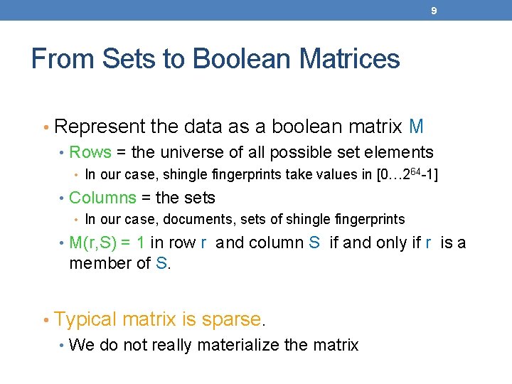
9 From Sets to Boolean Matrices • Represent the data as a boolean matrix M • Rows = the universe of all possible set elements • In our case, shingle fingerprints take values in [0… 264 -1] • Columns = the sets • In our case, documents, sets of shingle fingerprints • M(r, S) = 1 in row r and column S if and only if r is a member of S. • Typical matrix is sparse. • We do not really materialize the matrix

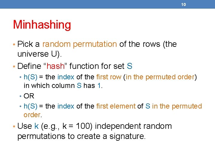
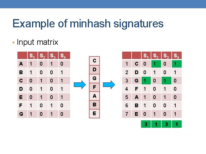
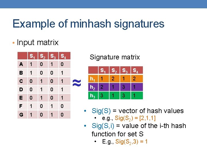
10 Minhashing • Pick a random permutation of the rows (the universe U). • Define “hash” function for set S • h(S) = the index of the first row (in the permuted order) in which column S has 1. • OR • h(S) = the index of the first element of S in the permuted order. • Use k (e. g. , k = 100) independent random permutations to create a signature.

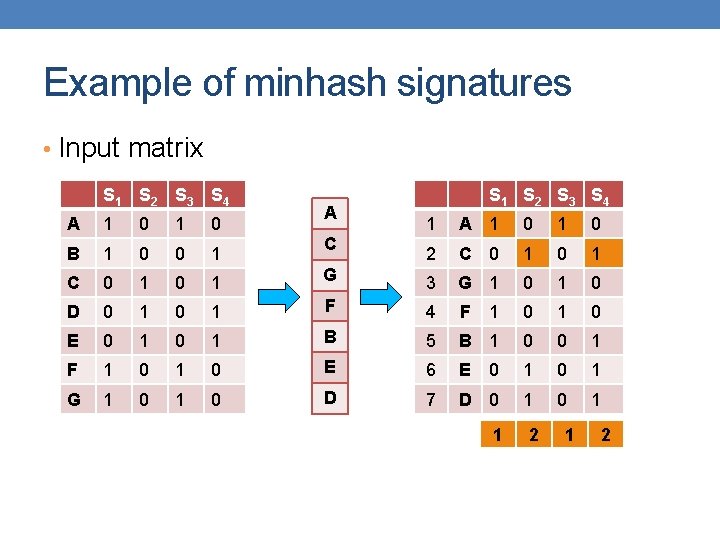
Example of minhash signatures • Input matrix S 1 S 2 S 3 S 4 A 1 0 B 1 0 0 1 C 0 1 D 0 1 0 E 0 1 F 1 G 1 A S 1 S 2 S 3 S 4 1 A 1 0 2 C 0 1 G 3 G 1 0 1 F 4 F 1 0 0 1 B 5 B 1 0 0 1 0 E 6 E 0 1 0 1 0 D 7 D 0 1 C 1 2

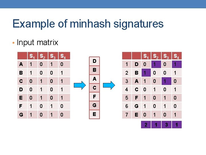
Example of minhash signatures • Input matrix S 1 S 2 S 3 S 4 A 1 0 B 1 0 0 1 C 0 1 D 0 1 0 E 0 1 F 1 G 1 D S 1 S 2 S 3 S 4 1 D 0 1 2 B 1 0 0 1 A 3 A 1 0 1 C 4 C 0 1 0 1 F 5 F 1 0 0 1 0 G 6 G 1 0 0 1 0 E 7 E 1 0 1 B 0 2 1 3 1

Example of minhash signatures • Input matrix S 1 S 2 S 3 S 4 A 1 0 B 1 0 0 1 C 0 1 D 0 1 0 E 0 1 F 1 G 1 C S 1 S 2 S 3 S 4 1 C 0 1 2 D 0 1 G 3 G 1 0 1 F 4 F 1 0 0 1 A 5 A 1 0 0 1 0 B 6 B 1 0 0 1 0 E 7 E 1 0 1 D 0 3 1

Example of minhash signatures • Input matrix S 1 S 2 S 3 S 4 A 1 0 B 1 0 0 1 C 0 1 D 0 1 E 0 1 F 1 0 G 1 0 Signature matrix ≈ S 1 S 2 S 3 S 4 h 1 1 2 h 2 2 1 3 1 h 3 3 1 • Sig(S) = vector of hash values • e. g. , Sig(S 2) = [2, 1, 1] • Sig(S, i) = value of the i-th hash function for set S • E. g. , Sig(S 2, 3) = 1

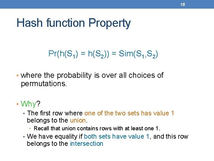
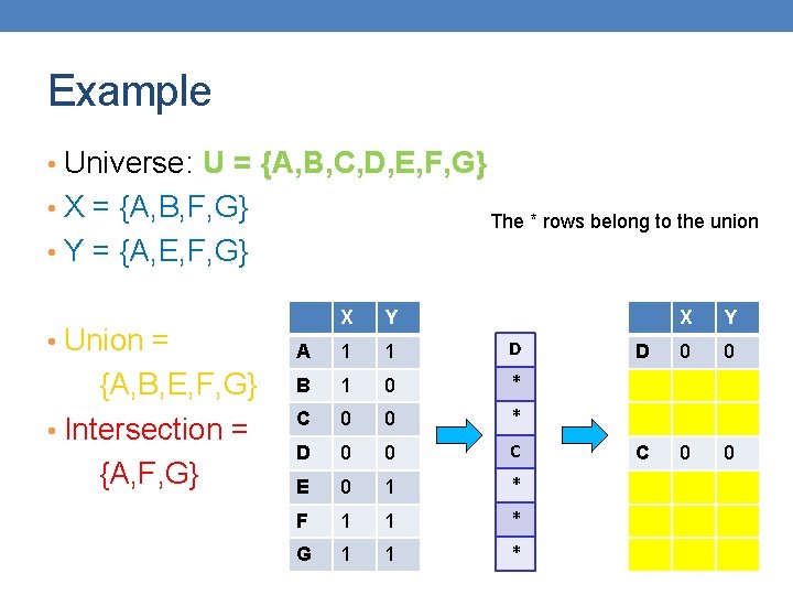
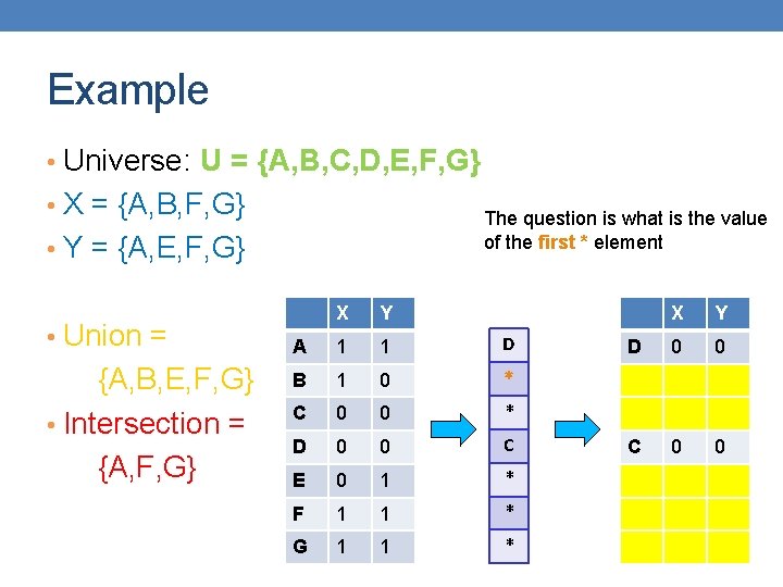
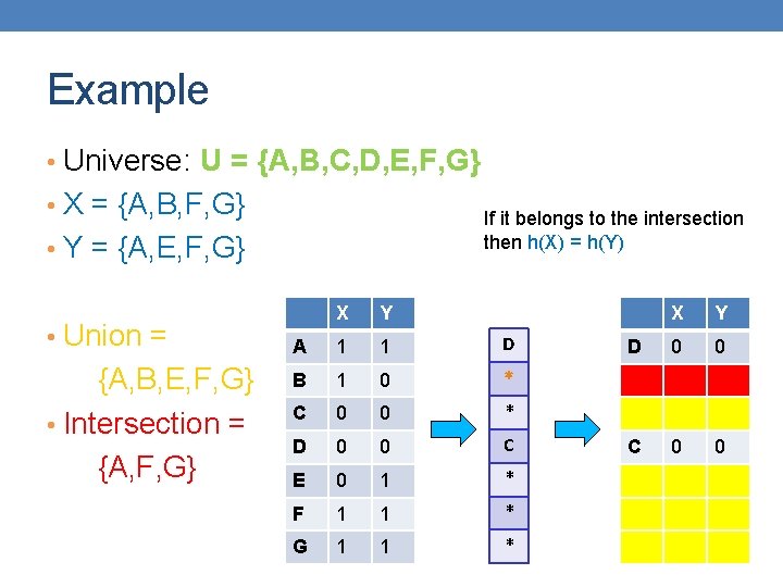
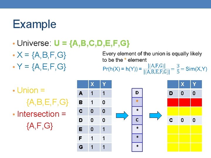
15 Hash function Property Pr(h(S 1) = h(S 2)) = Sim(S 1, S 2) • where the probability is over all choices of permutations. • Why? • The first row where one of the two sets has value 1 belongs to the union. • Recall that union contains rows with at least one 1. • We have equality if both sets have value 1, and this row belongs to the intersection

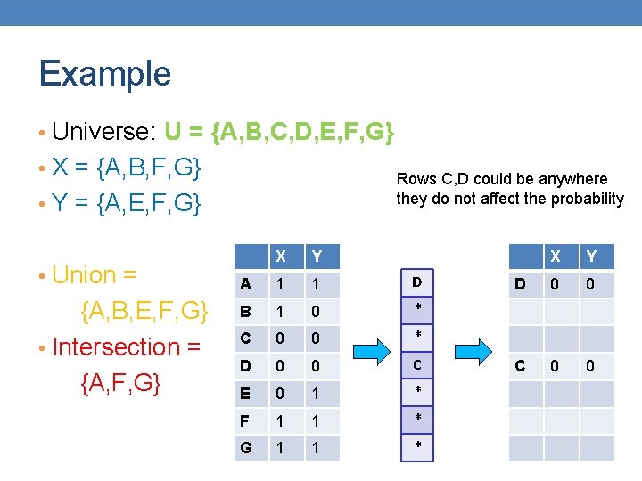
Example • Universe: U = {A, B, C, D, E, F, G} • X = {A, B, F, G} Rows C, D could be anywhere they do not affect the probability • Y = {A, E, F, G} • Union = {A, B, E, F, G} • Intersection = {A, F, G} X Y A 1 1 D B 1 0 * C 0 0 * D 0 0 C E 0 1 * F 1 1 * G 1 1 * X Y D 0 0 C 0 0

Example • Universe: U = {A, B, C, D, E, F, G} • X = {A, B, F, G} The * rows belong to the union • Y = {A, E, F, G} • Union = {A, B, E, F, G} • Intersection = {A, F, G} X Y A 1 1 D B 1 0 * C 0 0 * D 0 0 C E 0 1 * F 1 1 * G 1 1 * X Y D 0 0 C 0 0

Example • Universe: U = {A, B, C, D, E, F, G} • X = {A, B, F, G} The question is what is the value of the first * element • Y = {A, E, F, G} • Union = {A, B, E, F, G} • Intersection = {A, F, G} X Y A 1 1 D B 1 0 * C 0 0 * D 0 0 C E 0 1 * F 1 1 * G 1 1 * X Y D 0 0 C 0 0

Example • Universe: U = {A, B, C, D, E, F, G} • X = {A, B, F, G} If it belongs to the intersection then h(X) = h(Y) • Y = {A, E, F, G} • Union = {A, B, E, F, G} • Intersection = {A, F, G} X Y A 1 1 D B 1 0 * C 0 0 * D 0 0 C E 0 1 * F 1 1 * G 1 1 * X Y D 0 0 C 0 0

Example • Universe: U = {A, B, C, D, E, F, G} • X = {A, B, F, G} • Y = {A, E, F, G} • Union = {A, B, E, F, G} • Intersection = {A, F, G} X Y A 1 1 D B 1 0 * C 0 0 * D 0 0 C E 0 1 * F 1 1 * G 1 1 * X Y D 0 0 C 0 0

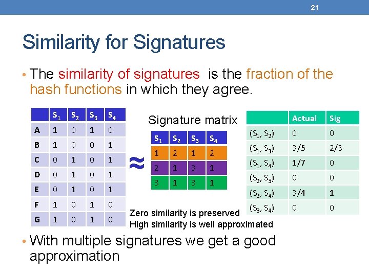
21 Similarity for Signatures • The similarity of signatures is the fraction of the hash functions in which they agree. S 1 S 2 S 3 S 4 A 1 0 B 1 0 0 1 C 0 1 D 0 1 E 0 1 F 1 0 G 1 0 Actual Sig (S 1, S 2) 0 0 (S 1, S 3) 3/5 2/3 (S 1, S 4) 1/7 0 (S 2, S 3) 0 0 (S 2, S 4) 3/4 1 0 0 Signature matrix ≈ S 1 S 2 S 3 S 4 1 2 2 1 3 1 3 1 (S 3, S 4) Zero similarity is preserved High similarity is well approximated • With multiple signatures we get a good approximation

Is it now feasible? • Assume a billion rows • Hard to pick a random permutation of 1…billion • Even representing a random permutation requires 1 billion entries!!! • How about accessing rows in permuted order?

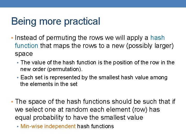
Being more practical • Instead of permuting the rows we will apply a hash function that maps the rows to a new (possibly larger) space • The value of the hash function is the position of the row in the new order (permutation). • Each set is represented by the smallest hash value among the elements in the set • The space of the hash functions should be such that if we select one at random each element (row) has equal probability to have the smallest value • Min-wise independent hash functions

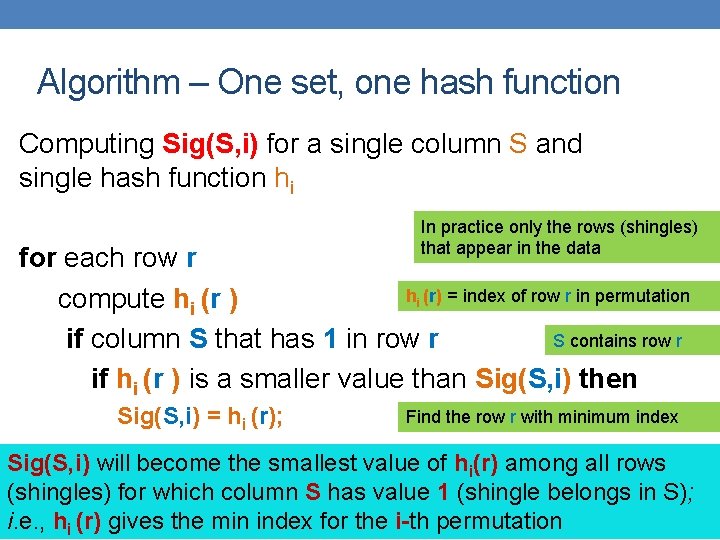
Algorithm – One set, one hash function Computing Sig(S, i) for a single column S and single hash function hi In practice only the rows (shingles) that appear in the data for each row r hi (r) = index of row r in permutation compute hi (r ) S contains row r if column S that has 1 in row r if hi (r ) is a smaller value than Sig(S, i) then Sig(S, i) = hi (r); Find the row r with minimum index Sig(S, i) will become the smallest value of hi(r) among all rows (shingles) for which column S has value 1 (shingle belongs in S); i. e. , hi (r) gives the min index for the i-th permutation

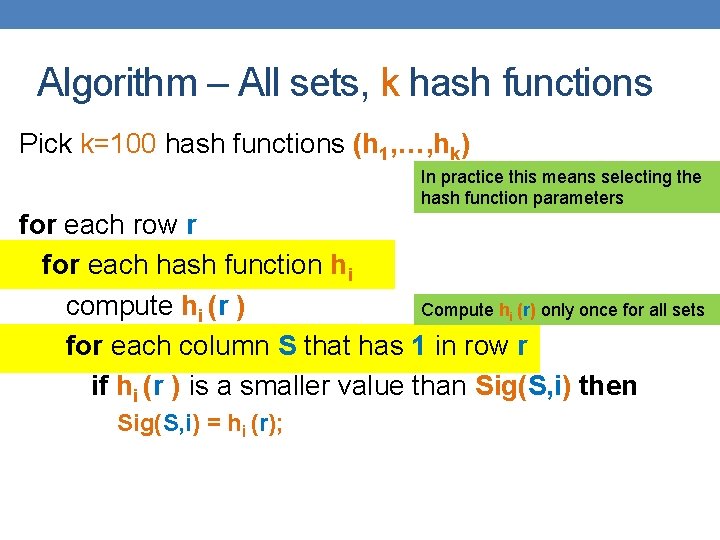
Algorithm – All sets, k hash functions Pick k=100 hash functions (h 1, …, hk) In practice this means selecting the hash function parameters for each row r for each hash function hi compute hi (r ) Compute hi (r) only once for all sets for each column S that has 1 in row r if hi (r ) is a smaller value than Sig(S, i) then Sig(S, i) = hi (r);

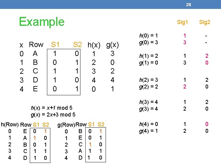
26 Example x 0 1 2 3 4 Row A B C D E S 1 1 0 Sig 1 S 2 h(x) g(x) 0 3 1 1 0 2 1 2 3 0 4 4 1 1 0 h(x) = x+1 mod 5 g(x) = 2 x+3 mod 5 h(Row) Row S 1 0 E 0 1 A 1 2 B 0 3 C 1 4 D 1 S 2 1 0 1 1 0 g(Row)Row S 1 0 B 0 1 E 0 2 C 1 3 A 1 4 D 1 S 2 1 1 0 1 0 Sig 2 h(0) = 1 g(0) = 3 1 3 - h(1) = 2 g(1) = 0 1 3 2 0 h(2) = 3 g(2) = 2 1 2 2 0 h(3) = 4 g(3) = 4 1 2 2 0 h(4) = 0 g(4) = 1 1 2 0 0

27 Implementation • Often, data is given by column, not row. • E. g. , columns = documents, rows = shingles. • If so, sort matrix once so it is by row. • And always compute hi (r ) only once for each row.

28 Finding similar pairs • Problem: Find all pairs of documents with similarity at least t = 0. 8 • While the signatures of all columns may fit in main memory, comparing the signatures of all pairs of columns is quadratic in the number of columns. • Example: 106 columns implies 5*1011 columncomparisons. • At 1 microsecond/comparison: 6 days.

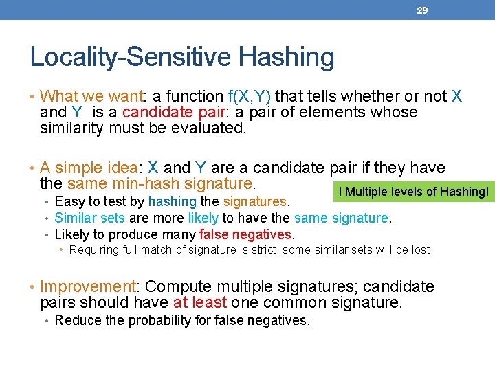
29 Locality-Sensitive Hashing • What we want: a function f(X, Y) that tells whether or not X and Y is a candidate pair: a pair of elements whose similarity must be evaluated. • A simple idea: X and Y are a candidate pair if they have the same min-hash signature. ! Multiple levels of Hashing! • Easy to test by hashing the signatures. • Similar sets are more likely to have the same signature. • Likely to produce many false negatives. • Requiring full match of signature is strict, some similar sets will be lost. • Improvement: Compute multiple signatures; candidate pairs should have at least one common signature. • Reduce the probability for false negatives.

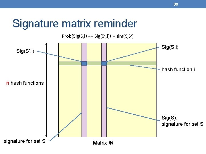
30 Signature matrix reminder Prob(Sig(S, i) == Sig(S’, i)) = sim(S, S’) Sig(S, i) Sig(S’, i) hash function i n hash functions Sig(S): signature for set S’ Matrix M

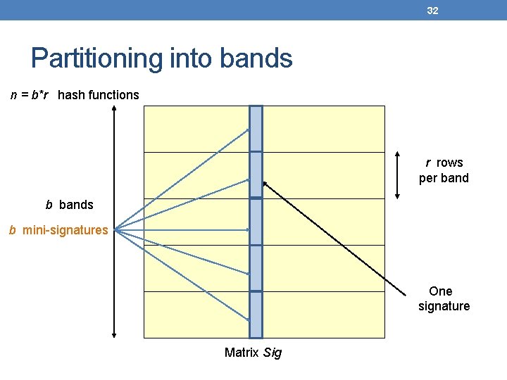
31 Partition into Bands – (1) • Divide the signature matrix Sig into b bands of r rows. • Each band is a mini-signature with r hash functions.

32 Partitioning into bands n = b*r hash functions r rows per band b bands b mini-signatures One signature Matrix Sig

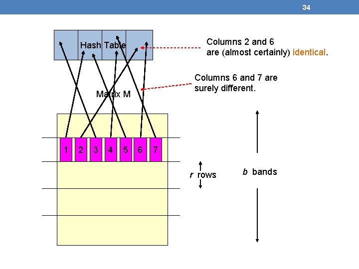
33 Partition into Bands – (2) • Divide the signature matrix Sig into b bands of r rows. • Each band is a mini-signature with r hash functions. • For each band, hash the mini-signature to a hash table with k buckets. • Make k as large as possible so that mini-signatures that hash to the same bucket are almost certainly identical.

34 Columns 2 and 6 are (almost certainly) identical. Hash Table Columns 6 and 7 are surely different. Matrix M 1 2 3 4 5 6 7 r rows b bands

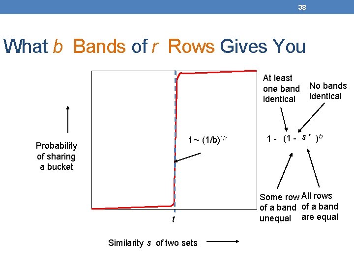
35 Partition into Bands – (3) • Divide the signature matrix Sig into b bands of r rows. • Each band is a mini-signature with r hash functions. • For each band, hash the mini-signature to a hash table with k buckets. • Make k as large as possible so that mini-signatures that hash to the same bucket are almost certainly identical. • Candidate column pairs are those that hash to the same bucket for at least 1 band. • Tune b and r to catch most similar pairs, but few nonsimilar pairs.

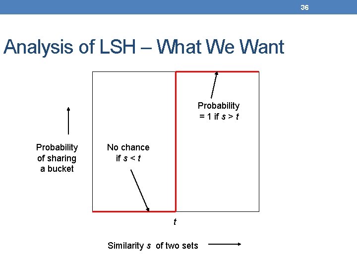
36 Analysis of LSH – What We Want Probability = 1 if s > t Probability of sharing a bucket No chance if s < t t Similarity s of two sets

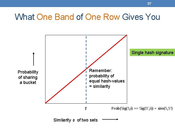
37 What One Band of One Row Gives You Single hash signature Remember: probability of equal hash-values = similarity Probability of sharing a bucket t Similarity s of two sets Prob(Sig(S, i) == Sig(S’, i)) = sim(S, S’)

38 What b Bands of r Rows Gives You At least one band identical t ~ (1/b)1/r Probability of sharing a bucket t Similarity s of two sets No bands identical 1 - (1 - s r )b Some row All rows of a band unequal are equal

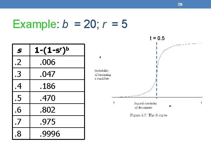
39 Example: b = 20; r = 5 t = 0. 5 s. 2. 3. 4. 5. 6. 7. 8 1 -(1 -sr)b. 006. 047. 186. 470. 802. 975. 9996

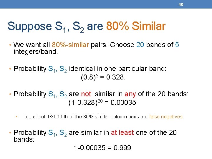
40 Suppose S 1, S 2 are 80% Similar • We want all 80%-similar pairs. Choose 20 bands of 5 integers/band. • Probability S 1, S 2 identical in one particular band: (0. 8)5 = 0. 328. • Probability S 1, S 2 are not similar in any of the 20 bands: (1 -0. 328)20 = 0. 00035 • i. e. , about 1/3000 -th of the 80%-similar column pairs are false negatives. • Probability S 1, S 2 are similar in at least one of the 20 bands: 1 -0. 00035 = 0. 999

41 Suppose S 1, S 2 Only 40% Similar • Probability S 1, S 2 identical in any one particular band: (0. 4)5 = 0. 01. • Probability S 1, S 2 identical in at least 1 of 20 bands: ≤ 20 * 0. 01 = 0. 2. • But false positives much lower for similarities << 40%.

42 LSH Summary • Tune to get almost all pairs with similar signatures, but eliminate most pairs that do not have similar signatures. • Check in main memory that candidate pairs really do have similar signatures. • Optional: In another pass through data, check that the remaining candidate pairs really represent similar sets.

Locality-sensitive hashing (LSH) • Big Picture: Construct hash functions h: Rd U such that for any pair of points p, q, for distance function D we have: • If D(p, q)≤r, then Pr[h(p)=h(q)] ≥ α is high • If D(p, q)≥cr, then Pr[h(p)=h(q)] ≤ β is small • Then, we can find close pairs by hashing • LSH is a general framework: for a given distance function D we need to find the right h • h is (r, cr, α, β)-sensitive

44 LSH for Cosine Distance • For cosine distance, there is a technique analogous to minhashing for generating a (d 1, d 2, (1 -d 1/180), (1 -d 2/180))- sensitive family for any d 1 and d 2. • Called random hyperplanes.

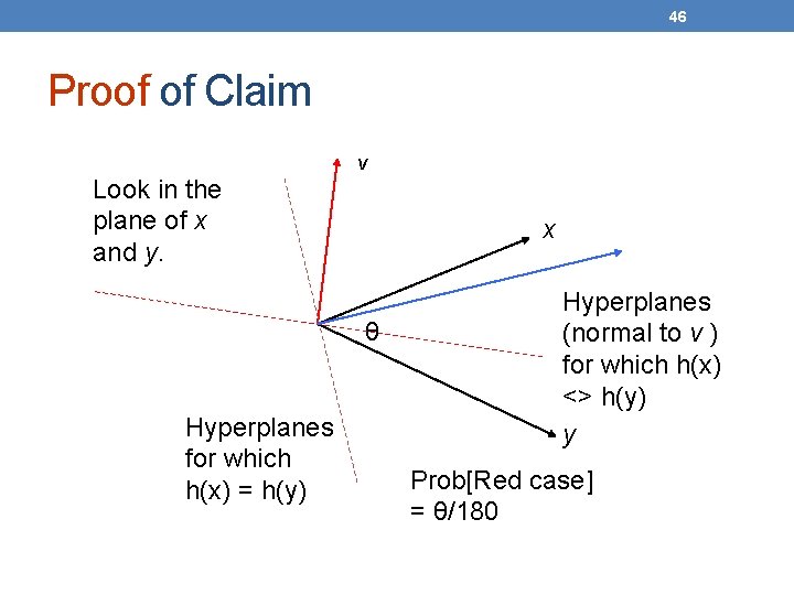
45 Random Hyperplanes • Pick a random vector v, which determines a hash function hv with two buckets. • hv(x) = +1 if v. x > 0; = -1 if v. x < 0. • LS-family H = set of all functions derived from any vector. • Claim: Prob[h(x)=h(y)] = 1 – (angle between x and y divided by 180).

46 Proof of Claim v Look in the plane of x and y. x θ Hyperplanes for which h(x) = h(y) Hyperplanes (normal to v ) for which h(x) <> h(y) y Prob[Red case] = θ/180

47 Signatures for Cosine Distance • Pick some number of vectors, and hash your data for each vector. • The result is a signature (sketch ) of +1’s and – 1’s that can be used for LSH like the minhash signatures for Jaccard distance.

48 Simplification • We need not pick from among all possible vectors v to form a component of a sketch. • It suffices to consider only vectors v consisting of +1 and – 1 components.

CLUSTERING

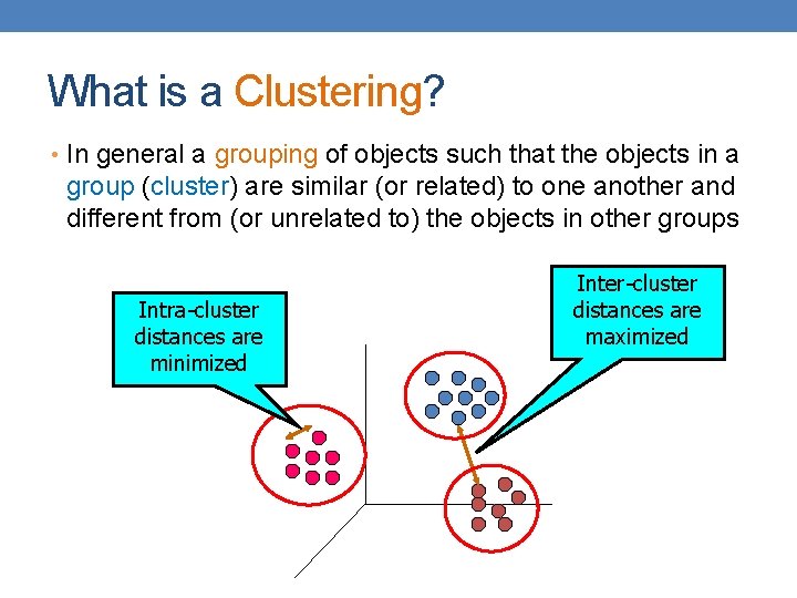
What is a Clustering? • In general a grouping of objects such that the objects in a group (cluster) are similar (or related) to one another and different from (or unrelated to) the objects in other groups Intra-cluster distances are minimized Inter-cluster distances are maximized

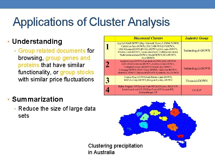
Applications of Cluster Analysis • Understanding • Group related documents for browsing, group genes and proteins that have similar functionality, or group stocks with similar price fluctuations • Summarization • Reduce the size of large data sets Clustering precipitation in Australia

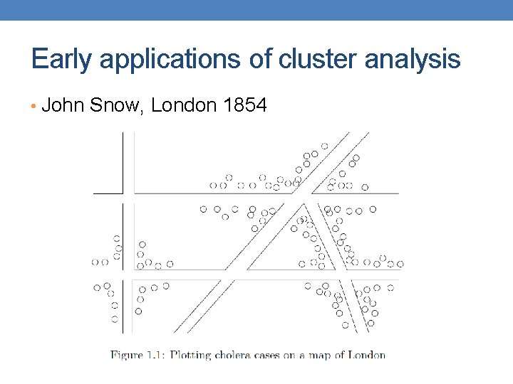
Early applications of cluster analysis • John Snow, London 1854

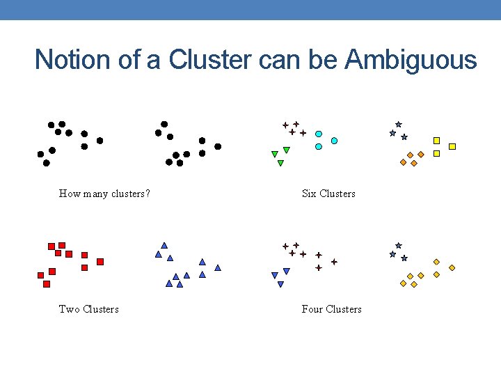
Notion of a Cluster can be Ambiguous How many clusters? Six Clusters Two Clusters Four Clusters

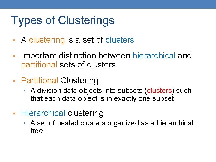
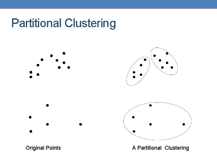
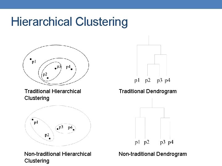
Types of Clusterings • A clustering is a set of clusters • Important distinction between hierarchical and partitional sets of clusters • Partitional Clustering • A division data objects into subsets (clusters) such that each data object is in exactly one subset • Hierarchical clustering • A set of nested clusters organized as a hierarchical tree

Partitional Clustering Original Points A Partitional Clustering

Hierarchical Clustering Traditional Dendrogram Non-traditional Hierarchical Clustering Non-traditional Dendrogram

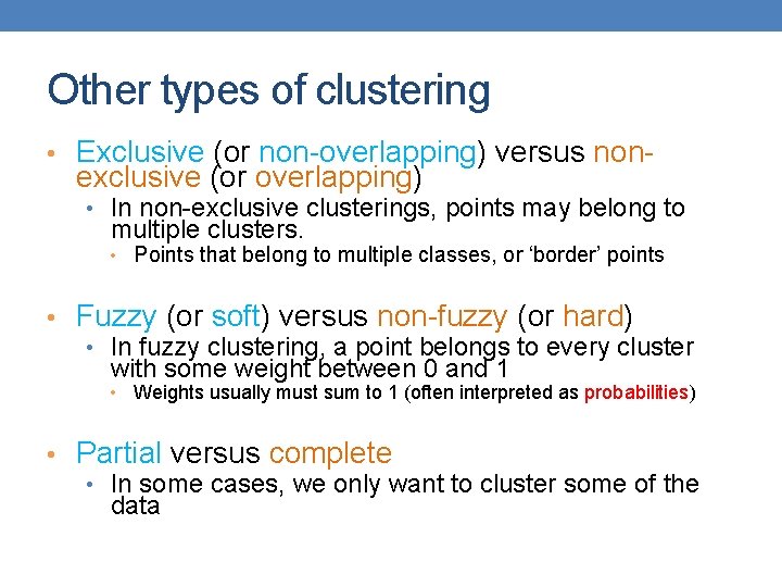
Other types of clustering • Exclusive (or non-overlapping) versus non- exclusive (or overlapping) • In non-exclusive clusterings, points may belong to multiple clusters. • Points that belong to multiple classes, or ‘border’ points • Fuzzy (or soft) versus non-fuzzy (or hard) • In fuzzy clustering, a point belongs to every cluster with some weight between 0 and 1 • Weights usually must sum to 1 (often interpreted as probabilities) • Partial versus complete • In some cases, we only want to cluster some of the data

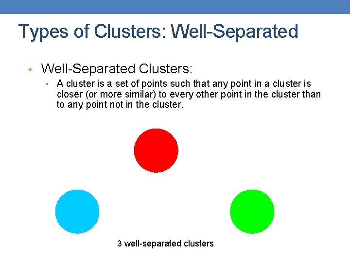
Types of Clusters: Well-Separated • Well-Separated Clusters: • A cluster is a set of points such that any point in a cluster is closer (or more similar) to every other point in the cluster than to any point not in the cluster. 3 well-separated clusters

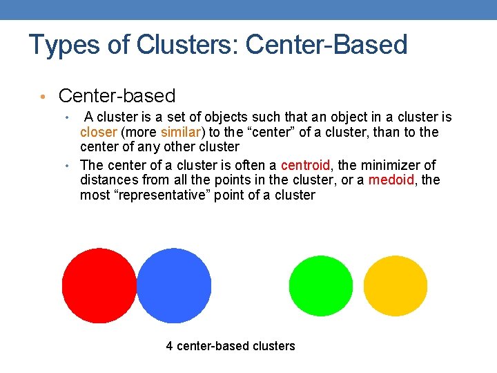
Types of Clusters: Center-Based • Center-based • A cluster is a set of objects such that an object in a cluster is closer (more similar) to the “center” of a cluster, than to the center of any other cluster • The center of a cluster is often a centroid, the minimizer of distances from all the points in the cluster, or a medoid, the most “representative” point of a cluster 4 center-based clusters

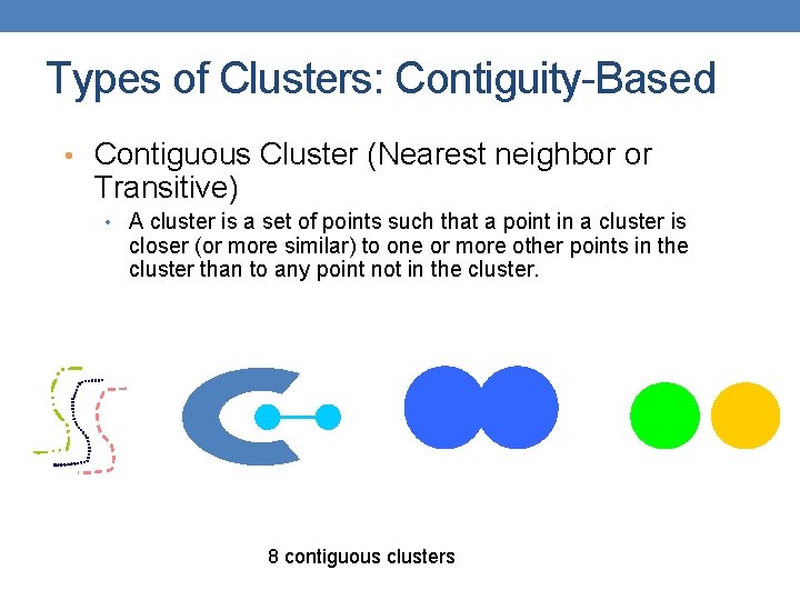
Types of Clusters: Contiguity-Based • Contiguous Cluster (Nearest neighbor or Transitive) • A cluster is a set of points such that a point in a cluster is closer (or more similar) to one or more other points in the cluster than to any point not in the cluster. 8 contiguous clusters

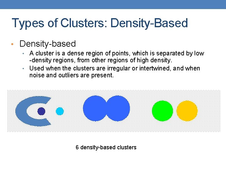
Types of Clusters: Density-Based • Density-based • A cluster is a dense region of points, which is separated by low -density regions, from other regions of high density. • Used when the clusters are irregular or intertwined, and when noise and outliers are present. 6 density-based clusters

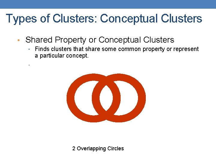
Types of Clusters: Conceptual Clusters • Shared Property or Conceptual Clusters • Finds clusters that share some common property or represent a particular concept. . 2 Overlapping Circles

Types of Clusters: Objective Function • Clustering as an optimization problem • Finds clusters that minimize or maximize an objective function. • Enumerate all possible ways of dividing the points into clusters and evaluate the `goodness' of each potential set of clusters by using the given objective function. (NP Hard) • Can have global or local objectives. • Hierarchical clustering algorithms typically have local objectives • Partitional algorithms typically have global objectives • A variation of the global objective function approach is to fit the data to a parameterized model. • The parameters for the model are determined from the data, and they determine the clustering • E. g. , Mixture models assume that the data is a ‘mixture' of a number of statistical distributions.

Clustering Algorithms • K-means and its variants • Hierarchical clustering • DBSCAN

K-MEANS

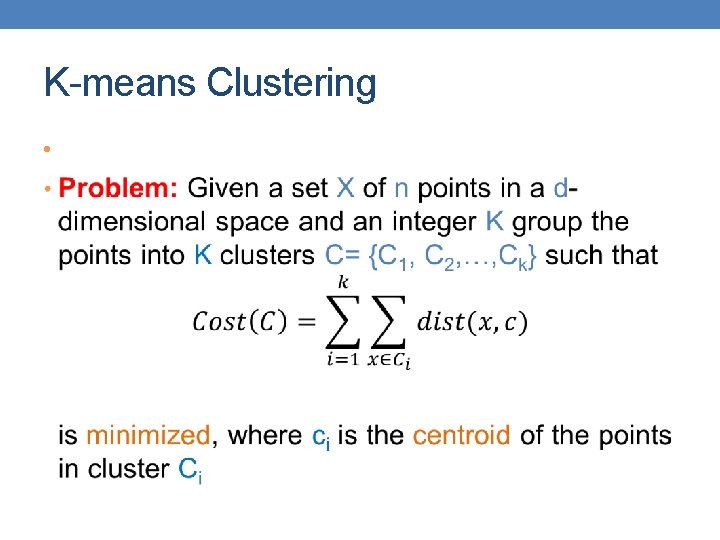
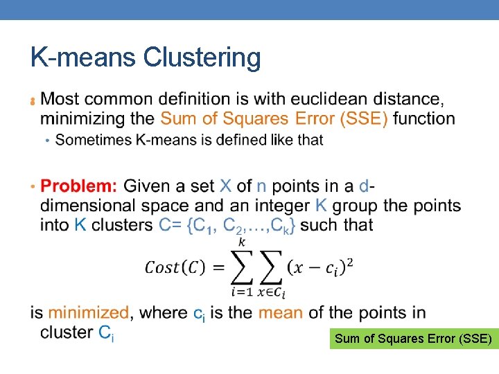
K-means Clustering • • • Partitional clustering approach Each cluster is associated with a centroid (center point) Each point is assigned to the cluster with the closest centroid Number of clusters, K, must be specified The objective is to minimize the sum of distances of the points to their respective centroid

K-means Clustering •

K-means Clustering • Sum of Squares Error (SSE)

Complexity of the k-means problem • NP-hard if the dimensionality of the data is at least 2 (d>=2) • Finding the best solution in polynomial time is infeasible • For d=1 the problem is solvable in polynomial time (how? ) • A simple iterative algorithm works quite well in practice

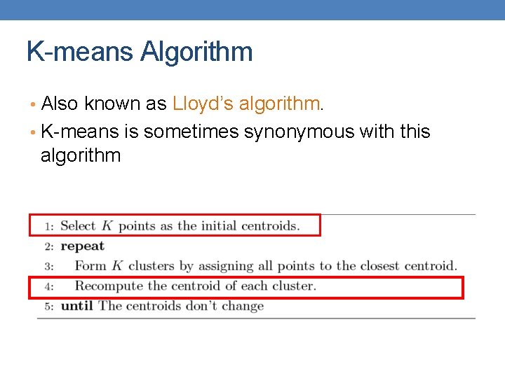
K-means Algorithm • Also known as Lloyd’s algorithm. • K-means is sometimes synonymous with this algorithm

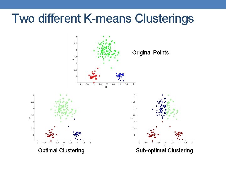
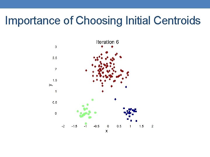
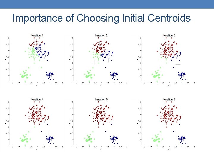
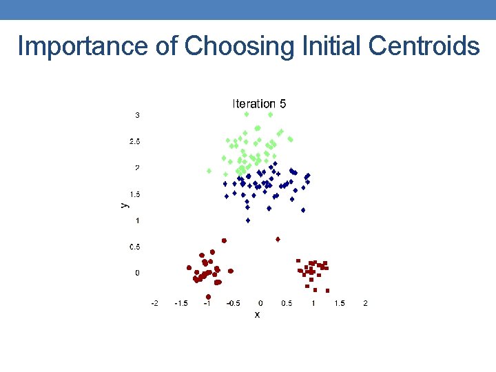
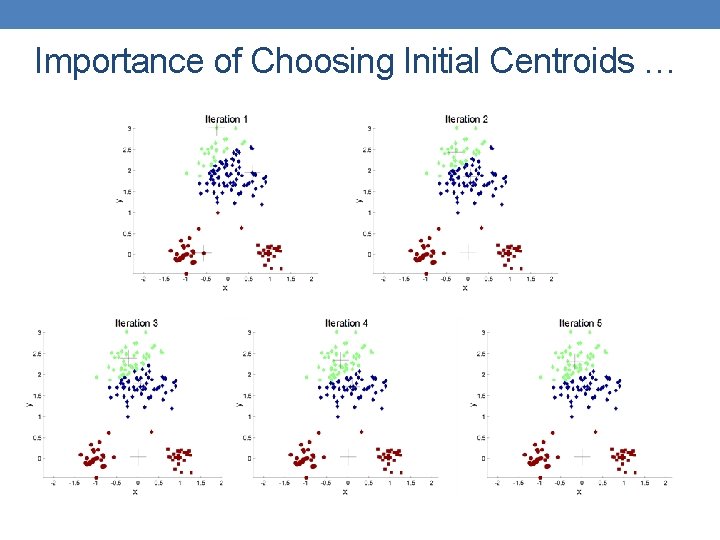
K-means Algorithm – Initialization • Initial centroids are often chosen randomly. • Clusters produced vary from one run to another.

Two different K-means Clusterings Original Points Optimal Clustering Sub-optimal Clustering

Importance of Choosing Initial Centroids

Importance of Choosing Initial Centroids

Importance of Choosing Initial Centroids

Importance of Choosing Initial Centroids …

Dealing with Initialization • Do multiple runs and select the clustering with the smallest error • Select original set of points by methods other than random. E. g. , pick the most distant (from each other) points as cluster centers (K-means++ algorithm)

K-means Algorithm – Centroids • The centroid depends on the distance function • The minimizer for the distance function • ‘Closeness’ is measured by Euclidean distance (SSE), cosine similarity, correlation, etc. • Centroid: • The mean of the points in the cluster for SSE, and cosine similarity • The median for Manhattan distance. • Finding the centroid is not always easy • It can be an NP-hard problem for some distance functions • E. g. , median form multiple dimensions

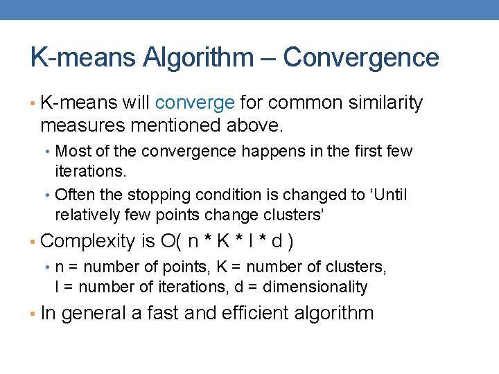
K-means Algorithm – Convergence • K-means will converge for common similarity measures mentioned above. • Most of the convergence happens in the first few iterations. • Often the stopping condition is changed to ‘Until relatively few points change clusters’ • Complexity is O( n * K * I * d ) • n = number of points, K = number of clusters, I = number of iterations, d = dimensionality • In general a fast and efficient algorithm

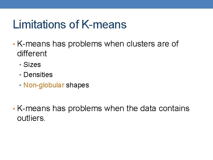
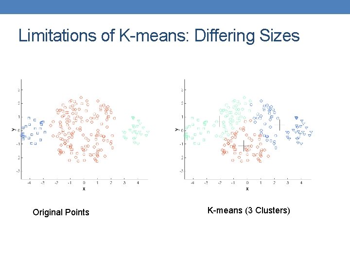
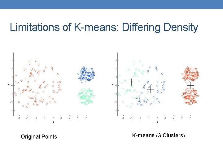
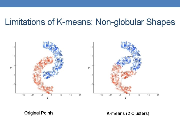
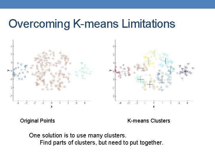
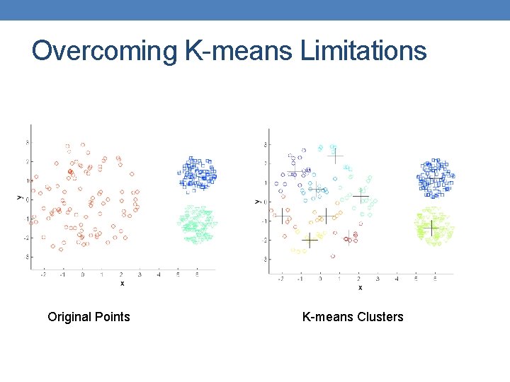
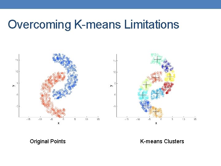
Limitations of K-means • K-means has problems when clusters are of different • Sizes • Densities • Non-globular shapes • K-means has problems when the data contains outliers.

Limitations of K-means: Differing Sizes Original Points K-means (3 Clusters)

Limitations of K-means: Differing Density Original Points K-means (3 Clusters)

Limitations of K-means: Non-globular Shapes Original Points K-means (2 Clusters)

Overcoming K-means Limitations Original Points K-means Clusters One solution is to use many clusters. Find parts of clusters, but need to put together.

Overcoming K-means Limitations Original Points K-means Clusters

Overcoming K-means Limitations Original Points K-means Clusters

Variations • K-medoids: Similar problem definition as in K- means, but the centroid of the cluster is defined to be one of the points in the cluster (the medoid). • K-centers: Similar problem definition as in K- means, but the goal now is to minimize the maximum diameter of the clusters (diameter of a cluster is maximum distance between any two points in the cluster).