DATA MINING LECTURE 11 Classification Support Vector Machines

Support Vector Machines • Find a linear hyperplane (decision boundary) that will separate the

Support Vector Machines • One Possible Solution

Support Vector Machines • Another possible solution

Support Vector Machines • Other possible solutions

Support Vector Machines • Which one is better? B 1 or B 2? •

Support Vector Machines • Find hyperplane maximizes the margin => B 1 is better

Support Vector Machines • We want to maximize: • Which is equivalent to minimizing:

Support Vector Machines • What if the problem is not linearly separable?

Support Vector Machines • What if the problem is not linearly separable? • Introduce

Nonlinear Support Vector Machines • What if decision boundary is not linear?

Nonlinear Support Vector Machines • Transform data into higher dimensional space Use the Kernel

Classification via regression • Instead of predicting the class of an record we want

Classification via regression • Assume a linear classification boundary

Logistic Regression The logistic function Linear regression on the log-odds ratio

Logistic Regression • Produces a probability estimate for the class membership which is often

Bayes Classifier • A probabilistic framework for solving classification problems • A, C random

Bayesian Classifiers • How to classify the new record X = (‘Yes’, ‘Single’, 80

Bayesian Classifiers • In order for probabilities to be well defined: • Consider each

Example • Record X = (Refund = Yes, Status = Single, Income =80 K)

How to Estimate Probabilities from Data? •

Example of Naïve Bayes Classifier • Creating a Naïve Bayes Classifier, essentially means to

Example of Naïve Bayes Classifier Given a Test Record: X = (Refund = Yes,

Example of Naïve Bayes Classifier With Laplace Smoothing Given a Test Record: X =

Naïve Bayes for Text Classification • Fraction of documents in c Laplace Smoothing Total

Example News titles for Politics and Sports Politics documents “Obama meets Merkel” “Obama elected

Naïve Bayes (Summary) • Robust to isolated noise points • Handle missing values by

Generative vs Discriminative models • Naïve Bayes is a type of a generative model

Generative vs Discriminative models • Logistic Regression and SVM are discriminative models • The

Learning • Supervised Learning: learn a model from the data using labeled data. •

Supervised Learning Steps • Model the problem • What is you are trying to

Modeling the problem • Sometimes it is not obvious. Consider the following three problems

Feature extraction • Feature extraction, or feature engineering is the most tedious but also

Training data • An overlooked problem: How do you get labeled data for training

Dealing with small amount of labeled data • Semi-supervised learning techniques have been developed

Technique • The choice of technique depends on the problem requirements (do we need

Big Data Trumps Better Algorithms • If you have enough data then the algorithms

Apply-Test • How do you scale to very large datasets? • Distributed computing –

Slides: 60

Download presentation

DATA MINING LECTURE 11 Classification Support Vector Machines Logistic Regression Naïve Bayes Classifier Supervised Learning

Illustrating Classification Task

SUPPORT VECTOR MACHINES

Support Vector Machines • Find a linear hyperplane (decision boundary) that will separate the data

Support Vector Machines • One Possible Solution

Support Vector Machines • Another possible solution

Support Vector Machines • Other possible solutions

Support Vector Machines • Which one is better? B 1 or B 2? • How do you define better?

Support Vector Machines • Find hyperplane maximizes the margin => B 1 is better than B 2

Support Vector Machines

Support Vector Machines • We want to maximize: • Which is equivalent to minimizing: • But subjected to the following constraints: • This is a constrained optimization problem • Numerical approaches to solve it (e. g. , quadratic programming)

Support Vector Machines • What if the problem is not linearly separable?

Support Vector Machines • What if the problem is not linearly separable? • Introduce slack variables • Need to minimize: • Subject to:

Nonlinear Support Vector Machines • What if decision boundary is not linear?

Nonlinear Support Vector Machines • Transform data into higher dimensional space Use the Kernel Trick

LOGISTIC REGRESSION

Classification via regression • Instead of predicting the class of an record we want to predict the probability of the class given the record • The problem of predicting continuous values is called regression problem • General approach: find a continuous function that models the continuous points.

Example: Linear regression •

Classification via regression • Assume a linear classification boundary

Logistic Regression The logistic function Linear regression on the log-odds ratio

Logistic Regression • Produces a probability estimate for the class membership which is often very useful. • The weights can be useful for understanding the feature importance. • Works for relatively large datasets • Fast to apply.

NAÏVE BAYES CLASSIFIER

Bayes Classifier • A probabilistic framework for solving classification problems • A, C random variables • Joint probability: Pr(A=a, C=c) • Conditional probability: Pr(C=c | A=a) • Relationship between joint and conditional probability distributions • Bayes Theorem:

Bayesian Classifiers • How to classify the new record X = (‘Yes’, ‘Single’, 80 K) Find the class with the highest probability given the vector values. Maximum Aposteriori Probability estimate: • Find the value c for class C that maximizes P(C=c| X) How do we estimate P(C|X) for the different values of C? • We want to estimate P(C=Yes| X) • and P(C=No| X)

Bayesian Classifiers • In order for probabilities to be well defined: • Consider each attribute and the class label as random variables • Probabilities are determined from the data Evade C Event space: {Yes, No} P(C) = (0. 3, 0. 7) Refund A 1 Event space: {Yes, No} P(A 1) = (0. 3, 0. 7) Martial Status A 2 Event space: {Single, Married, Divorced} P(A 2) = (0. 4, 0. 2) Taxable Income A 3 Event space: R P(A 3) ~ Normal( , 2) μ = 104: sample mean, 2=1874: sample var

Bayesian Classifiers •

Naïve Bayes Classifier •

How to Estimate Probabilities from Data? •

Example of Naïve Bayes Classifier • Creating a Naïve Bayes Classifier, essentially means to compute counts: Total number of records: N = 10 Class No: Number of records: 7 Attribute Refund: Yes: 3 No: 4 Attribute Marital Status: Single: 2 Divorced: 1 Married: 4 Attribute Income: mean: 110 variance: 2975 Class Yes: Number of records: 3 Attribute Refund: Yes: 0 No: 3 Attribute Marital Status: Single: 2 Divorced: 1 Married: 0 Attribute Income: mean: 90 variance: 25

Naïve Bayes Classifier •

Implementation details •

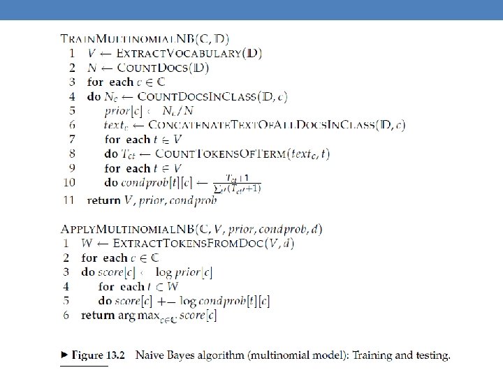
Naïve Bayes for Text Classification • Fraction of documents in c Laplace Smoothing Total number of terms in all documents in c Number of unique words (vocabulary size)

Multinomial document model • w

Example News titles for Politics and Sports Politics documents “Obama meets Merkel” “Obama elected again” “Merkel visits Greece again” P(p) = 0. 5 obama: 2, meets: 1, merkel: 2, Vocabulary elected: 1, again: 2, visits: 1, greece: 1 size: 14 terms Total terms: 10 New title: Sports “OSFP European basketball champion” “Miami NBA basketball champion” “Greece basketball coach? ” P(s) = 0. 5 OSFP: 1, european: 1, basketball: 3, champion: 2, miami: 1, nba: 1, greece: 1, coach: 1 Total terms: 11 X = “Obama likes basketball” P(Politics|X) ~ P(p)*P(obama|p)*P(likes|p)*P(basketball|p) = 0. 5 * 3/(10+14) *1/(10+14) * 1/(10+14) = 0. 000108 P(Sports|X) ~ P(s)*P(obama|s)*P(likes|s)*P(basketball|s) = 0. 5 * 1/(11+14) * 4/(11+14) = 0. 000128

Naïve Bayes (Summary) • Robust to isolated noise points • Handle missing values by ignoring the instance during probability estimate calculations • Robust to irrelevant attributes • Independence assumption may not hold for some attributes • Use other techniques such as Bayesian Belief Networks (BBN) • Naïve Bayes can produce a probability estimate, but it is usually a very biased one • Logistic Regression is better for obtaining probabilities.

Generative vs Discriminative models • Naïve Bayes is a type of a generative model • Generative process: • First pick the category of the record • Then given the category, generate the attribute values from the distribution of the category • Conditional independence given C C • We use the training data to learn the distribution of the values in a class

Generative vs Discriminative models • Logistic Regression and SVM are discriminative models • The goal is to find the boundary that discriminates between the two classes from the training data • In order to classify the language of a document, you can • Either learn the two languages and find which is more likely to have generated the words you see • Or learn what differentiates the two languages.

SUPERVISED LEARNING

Learning • Supervised Learning: learn a model from the data using labeled data. • Classification and Regression are the prototypical examples of supervised learning tasks. Other are possible (e. g. , ranking) • Unsupervised Learning: learn a model – extract structure from unlabeled data. • Clustering and Association Rules are prototypical examples of unsupervised learning tasks. • Semi-supervised Learning: learn a model for the data using both labeled and unlabeled data.

Supervised Learning Steps • Model the problem • What is you are trying to predict? What kind of optimization function do you need? Do you need classes or probabilities? • Extract Features • How do you find the right features that help to discriminate between the classes? • Obtain training data • Obtain a collection of labeled data. Make sure it is large enough, accurate and representative. Ensure that classes are well represented. • Decide on the technique • What is the right technique for your problem? • Apply in practice • Can the model be trained for very large data? How do you test how you do in practice? How do you improve?

Modeling the problem • Sometimes it is not obvious. Consider the following three problems • Detecting if an email is spam • Categorizing the queries in a search engine • Ranking the results of a web search

Feature extraction • Feature extraction, or feature engineering is the most tedious but also the most important step • How do you separate the players of the Greek national team from those of the Swedish national team? • One line of thought: throw features to the classifier and the classifier will figure out which ones are important • More features, means that you need more training data • Another line of thought: Feature Selection: Select carefully the features using various functions and techniques • Computationally intensive

Training data • An overlooked problem: How do you get labeled data for training your model? • E. g. , how do you get training data for ranking? • Usually requires a lot of manual effort and domain expertise and carefully planned labeling • Results are not always of high quality (lack of expertise) • And they are not sufficient (low coverage of the space) • Recent trends: • Find a source that generates the labeled data for you. • Crowd-sourcing techniques

Dealing with small amount of labeled data • Semi-supervised learning techniques have been developed for this purpose. • Self-training: Train a classifier on the data, and then feed back the high-confidence output of the classifier as input • Co-training: train two “independent” classifiers and feed the output of one classifier as input to the other. • Regularization: Treat learning as an optimization problem where you define relationships between the objects you want to classify, and you exploit these relationships • Example: Image restoration

Technique • The choice of technique depends on the problem requirements (do we need a probability estimate? ) and the problem specifics (does independence assumption hold? do we think classes are linearly separable? ) • For many cases finding the right technique may be trial and error • For many cases the exact technique does not matter.

Big Data Trumps Better Algorithms • If you have enough data then the algorithms are not so important • The web has made this possible. • Especially for text-related tasks • Search engine uses the collective human intelligence Google lecture: Theorizing from the Data

Apply-Test • How do you scale to very large datasets? • Distributed computing – map-reduce implementations of machine learning algorithms (Mahut, over Hadoop) • How do you test something that is running online? • You cannot get labeled data in this case • A/B testing • How do you deal with changes in data? • Active learning