Data Mining Engineering Input and Output Chapter 7

Data Mining – Engineering Input and Output Chapter 7

Performance Estimation and Parameter Tuning • If you compare approaches using 10 -fold cross validation, and vary parameters to see which comes out best … – You are performing human-assisted machine learning and essentially peeking at the test data as part of your learniing – Performance by best approach probably overestimates performance on a completely new, never before seen set of data

Engineering Input • Attribute selection • Attribute discretization • The test during learning cannot be done on training data or test data • Data cleansing • Creation of new “synthetic” attributes – E. g. combination of two or more attributes

Attribute Selection • Some attributes are irrelevant – adding irrelevant attributes “distract” or “confuse” machine learning schemes – Divide and conquer approaches end up at some point dealing with a small number of instances, where coincidences with irrelevant attributes may seem significant – Same with instance based approaches – Naïve Bayes is immune since it looks at all instances and all attributes and assumes independence – perfect for an irrelevant attribute – since it IS independent

Attribute Selection • Some attributes are redundant with other attributes – Leads Naïve Bayes and linear regression astray

Attribute Selection • Removing irrelevant or redundant attributes – Increases performance (not necessarily dramatically) – Speeds learning – Likely results in a simpler model (e. g. smaller decision tree; fewer or shorter rules)

Attribute Selection • Best approach – select relevant attributes manually, using human knowledge and experience (assuming that you are not RESEARCHING automatic attribute selection) • Much research has addressed attribute selection • WEKA has several approaches supported • We will discuss several approaches

Filter vs Wrapper • Two fundamentally different approaches • Filter – based on analysis of data independent of any learning algorithm to be used – data set is filtered in advance • Wrapper – evaluate which attributes should be used using the machine learning algorithm that will be used – the learning method is wrapped inside the selection procedure

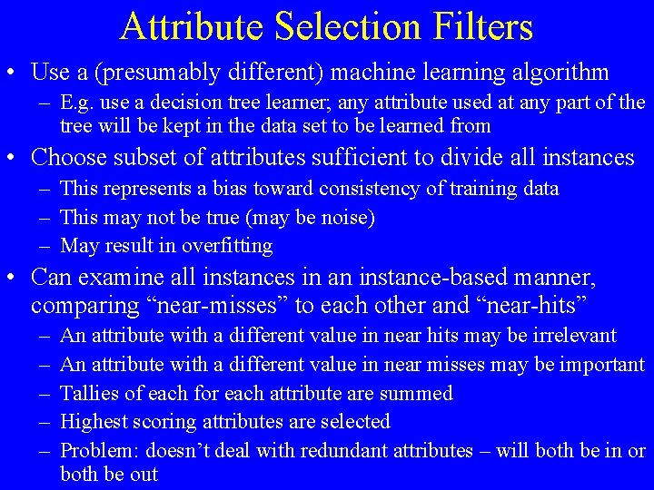
Attribute Selection Filters • Use a (presumably different) machine learning algorithm – E. g. use a decision tree learner; any attribute used at any part of the tree will be kept in the data set to be learned from • Choose subset of attributes sufficient to divide all instances – This represents a bias toward consistency of training data – This may not be true (may be noise) – May result in overfitting • Can examine all instances in an instance-based manner, comparing “near-misses” to each other and “near-hits” – – – An attribute with a different value in near hits may be irrelevant An attribute with a different value in near misses may be important Tallies of each for each attribute are summed Highest scoring attributes are selected Problem: doesn’t deal with redundant attributes – will both be in or both be out

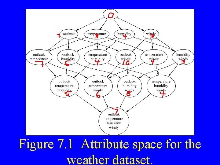
Searching the Attribute Space • Most filter approaches involve searching the space of attributes for the subset that is most likely to predict the class best • See next slide – shows the space of possible attribute subsets for the weather data

Figure 7. 1 Attribute space for the weather dataset.

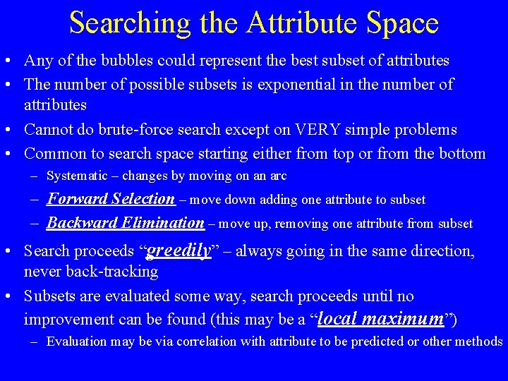
Searching the Attribute Space • Any of the bubbles could represent the best subset of attributes • The number of possible subsets is exponential in the number of attributes • Cannot do brute-force search except on VERY simple problems • Common to search space starting either from top or from the bottom – Systematic – changes by moving on an arc – Forward Selection – move down adding one attribute to subset – Backward Elimination – move up, removing one attribute from subset • Search proceeds “greedily” – always going in the same direction, never back-tracking • Subsets are evaluated some way, search proceeds until no improvement can be found (this may be a “local maximum”) – Evaluation may be via correlation with attribute to be predicted or other methods

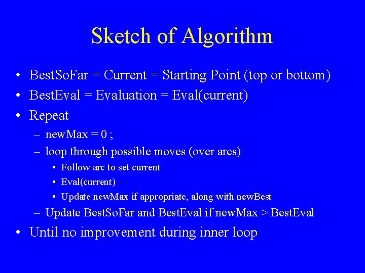
Sketch of Algorithm • Best. So. Far = Current = Starting Point (top or bottom) • Best. Eval = Evaluation = Eval(current) • Repeat – new. Max = 0 ; – loop through possible moves (over arcs) • Follow arc to set current • Eval(current) • Update new. Max if appropriate, along with new. Best – Update Best. So. Far and Best. Eval if new. Max > Best. Eval • Until no improvement during inner loop

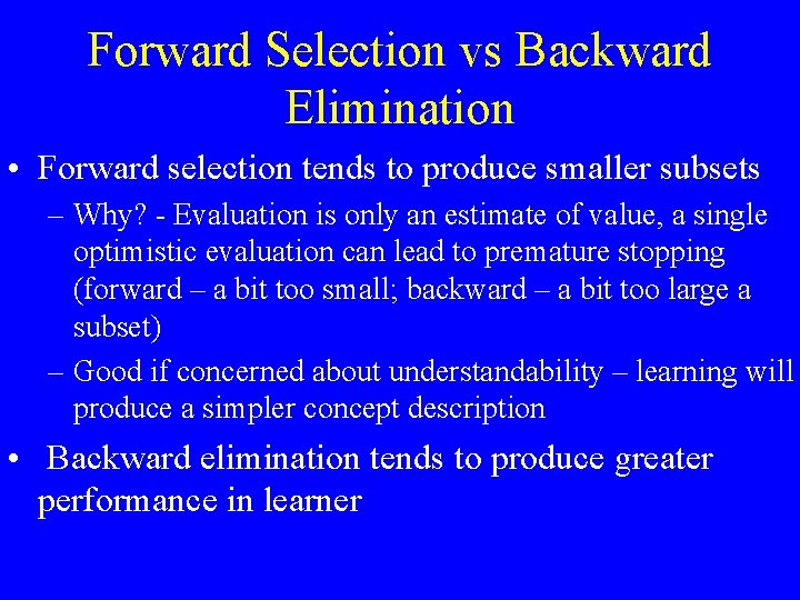
Forward Selection vs Backward Elimination • Forward selection tends to produce smaller subsets – Why? - Evaluation is only an estimate of value, a single optimistic evaluation can lead to premature stopping (forward – a bit too small; backward – a bit too large a subset) – Good if concerned about understandability – learning will produce a simpler concept description • Backward elimination tends to produce greater performance in learner

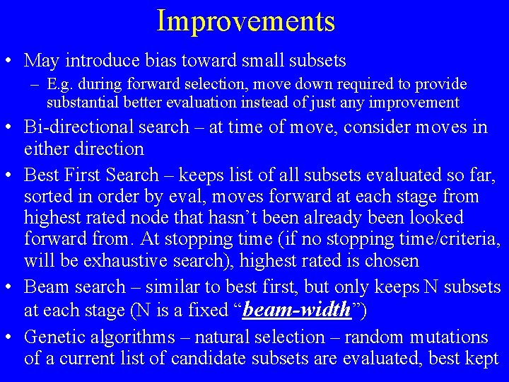
Improvements • May introduce bias toward small subsets – E. g. during forward selection, move down required to provide substantial better evaluation instead of just any improvement • Bi-directional search – at time of move, consider moves in either direction • Best First Search – keeps list of all subsets evaluated so far, sorted in order by eval, moves forward at each stage from highest rated node that hasn’t been already been looked forward from. At stopping time (if no stopping time/criteria, will be exhaustive search), highest rated is chosen • Beam search – similar to best first, but only keeps N subsets at each stage (N is a fixed “beam-width”) • Genetic algorithms – natural selection – random mutations of a current list of candidate subsets are evaluated, best kept

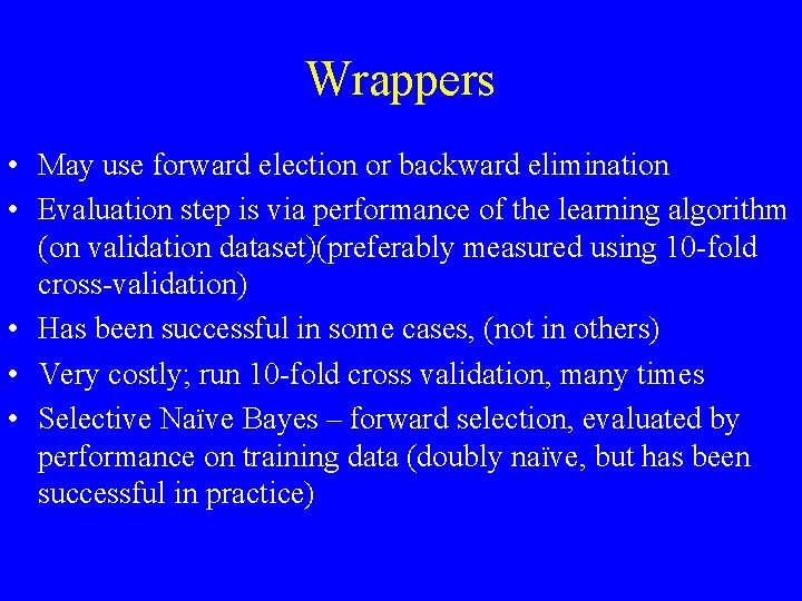
Wrappers • May use forward election or backward elimination • Evaluation step is via performance of the learning algorithm (on validation dataset)(preferably measured using 10 -fold cross-validation) • Has been successful in some cases, (not in others) • Very costly; run 10 -fold cross validation, many times • Selective Naïve Bayes – forward selection, evaluated by performance on training data (doubly naïve, but has been successful in practice)

7. 2 Attribute Discretization • Some algorithms cannot handle numeric attributes • Some algorithms may perform better without numeric attributes • Some algorithms may be more efficient without numeric attributes • One approach was discussed when discussing One. R • NOTE – it may be useful to go part way – to ordered categories

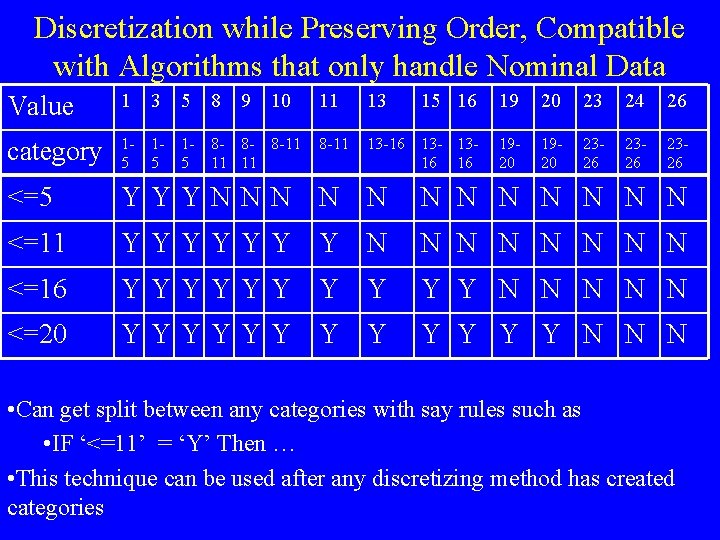
Discretization while Preserving Order, Compatible with Algorithms that only handle Nominal Data Value 1 3 5 8 9 10 11 13 15 16 19 20 23 24 26 category 15 15 15 8 - 8 - 8 -11 11 11 8 -11 13 -16 13 - 1316 16 1920 2326 <=5 YYYNNN N N N N <=11 YYYYYY Y N N N N <=16 YYYYYY Y Y N N N <=20 YYYYYY Y Y Y N N N • Can get split between any categories with say rules such as • IF ‘<=11’ = ‘Y’ Then … • This technique can be used after any discretizing method has created categories

Supervised vs Unsupervised • One. R’s discretization is supervised – class is considered • Unsupervised – only values for the attribute being discretized are considered. • Supervised can be beneficial because divisions may later help the learning method – by providing an attribute that helps to divide classes

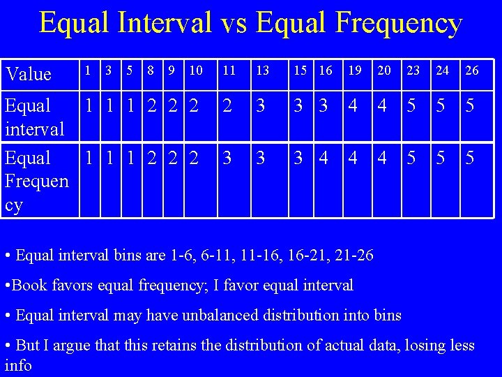
Unsupervised • Equal-Interval Binning - Divide range on the attribute into N subranges (based on how many categories (or bins) are desired) • Equal-Frequency Binning – divide range into N subranges such that each subrange has the same number of instances in it

Equal Interval vs Equal Frequency 10 11 13 15 16 19 20 23 24 26 Equal 1 1 1 2 2 2 interval Equal 1 1 1 2 2 2 Frequen cy 2 3 3 3 4 4 5 5 5 3 3 3 4 4 4 5 5 5 Value 1 3 5 8 9 • Equal interval bins are 1 -6, 6 -11, 11 -16, 16 -21, 21 -26 • Book favors equal frequency; I favor equal interval • Equal interval may have unbalanced distribution into bins • But I argue that this retains the distribution of actual data, losing less info

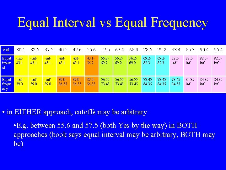
Equal Interval vs Equal Frequency Val 30. 1 32. 5 37. 5 40. 5 42. 6 55. 6 57. 5 67. 4 68. 4 78. 5 79. 2 83. 4 85. 3 90. 4 95. 4 Equal interv al -inf 43. 156. 269. 282. 3 inf 82. 3 inf Equal freque ncy -inf 39. 056. 55 39. 056. 5573. 45 56. 5573. 4584. 35 73. 4584. 35 inf 84. 35 inf • in EITHER approach, cutoffs may be arbitrary • E. g. between 55. 6 and 57. 5 (both Yes by the way) in BOTH approaches (book says equal interval may be arbitrary, BOTH may be)

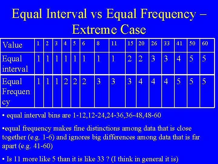
Equal Interval vs Equal Frequency – Extreme Case 6 8 11 15 20 26 33 41 50 60 Equal 1 1 1 interval Equal 1 1 1 2 2 2 Frequen cy 1 1 2 2 3 3 4 5 5 3 3 3 4 4 4 5 5 5 Value 1 2 3 4 5 • equal interval bins are 1 -12, 12 -24, 24 -36, 36 -48, 48 -60 • equal frequency makes fine distinctions among data that is close together (e. g. 1 -6) and ignores big differences among data that is far apart (e. g. 41 -60) • Is 11 more like 5 than it is like 33 ? (I think in general it is)

Not in Book - Other Possibilities for Unsupervised • Clustering • Gap finding

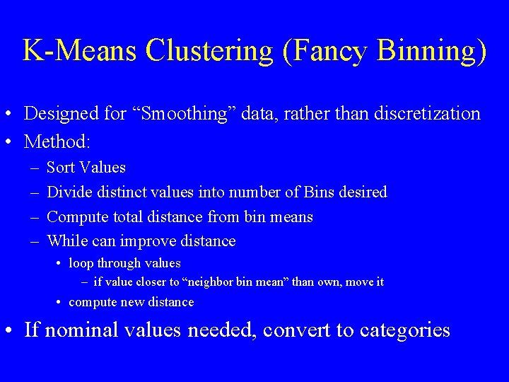
K-Means Clustering (Fancy Binning) • Designed for “Smoothing” data, rather than discretization • Method: – – Sort Values Divide distinct values into number of Bins desired Compute total distance from bin means While can improve distance • loop through values – if value closer to “neighbor bin mean” than own, move it • compute new distance • If nominal values needed, convert to categories

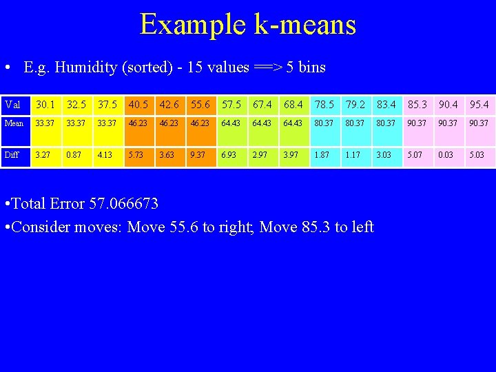
Example k-means • E. g. Humidity (sorted) - 15 values ==> 5 bins Val 30. 1 32. 5 37. 5 40. 5 42. 6 55. 6 57. 5 67. 4 68. 4 78. 5 79. 2 83. 4 85. 3 90. 4 95. 4 Mean 33. 37 46. 23 64. 43 80. 37 90. 37 Diff 3. 27 0. 87 4. 13 5. 73 3. 63 9. 37 6. 93 2. 97 3. 97 1. 87 1. 17 3. 03 5. 07 0. 03 5. 03 • Total Error 57. 066673 • Consider moves: Move 55. 6 to right; Move 85. 3 to left

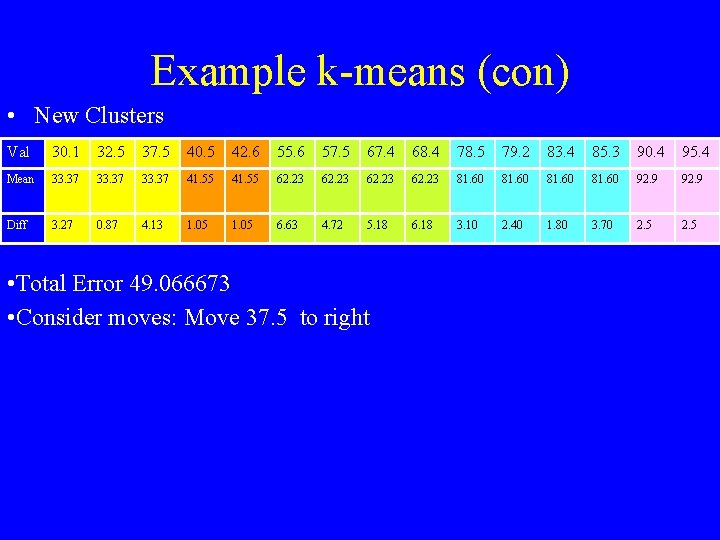
Example k-means (con) • New Clusters Val 30. 1 32. 5 37. 5 40. 5 42. 6 55. 6 57. 5 67. 4 68. 4 78. 5 79. 2 83. 4 85. 3 90. 4 95. 4 Mean 33. 37 41. 55 62. 23 81. 60 92. 9 Diff 3. 27 0. 87 4. 13 1. 05 6. 63 4. 72 5. 18 6. 18 3. 10 2. 40 1. 80 3. 70 2. 5 • Total Error 49. 066673 • Consider moves: Move 37. 5 to right

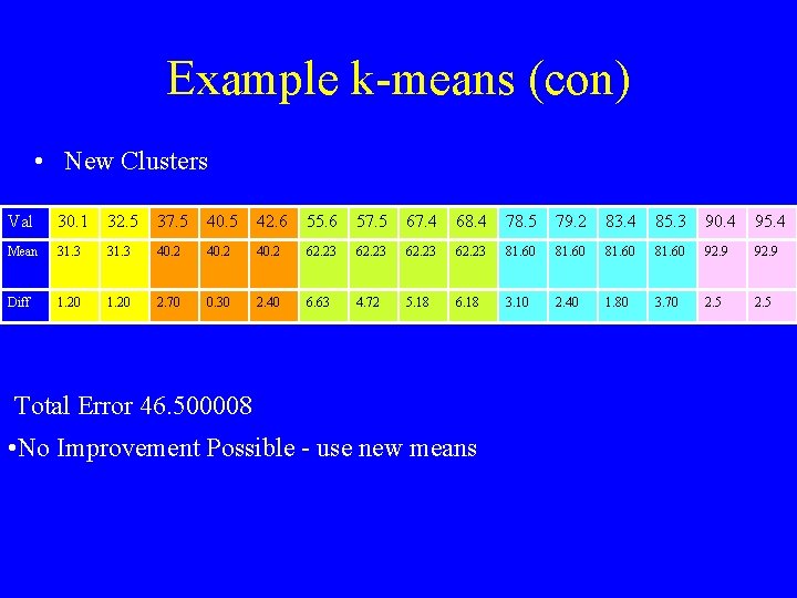
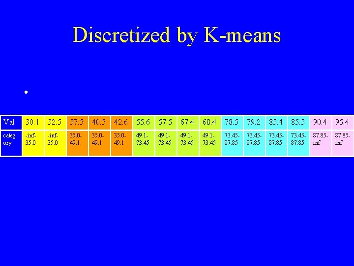
Example k-means (con) • New Clusters Val 30. 1 32. 5 37. 5 40. 5 42. 6 55. 6 57. 5 67. 4 68. 4 78. 5 79. 2 83. 4 85. 3 90. 4 95. 4 Mean 31. 3 40. 2 62. 23 81. 60 92. 9 Diff 1. 20 2. 70 0. 30 2. 40 6. 63 4. 72 5. 18 6. 18 3. 10 2. 40 1. 80 3. 70 2. 5 Total Error 46. 500008 • No Improvement Possible - use new means

Discretized by K-means • Val 30. 1 32. 5 37. 5 40. 5 42. 6 55. 6 57. 5 67. 4 68. 4 78. 5 79. 2 83. 4 85. 3 90. 4 95. 4 categ ory -inf 35. 049. 1 35. 049. 173. 45 49. 173. 4587. 85 73. 4587. 85 inf

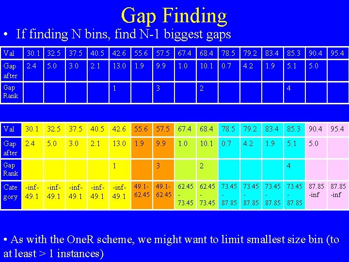
Gap Finding • If finding N bins, find N-1 biggest gaps Val 30. 1 32. 5 37. 5 40. 5 42. 6 55. 6 57. 5 67. 4 68. 4 78. 5 79. 2 83. 4 85. 3 90. 4 Gap after 2. 4 3. 0 2. 1 13. 0 1. 9 9. 9 1. 0 10. 1 0. 7 4. 2 1. 9 5. 1 5. 0 Gap Rank Val 1 30. 1 Gap 2. 4 after 2 4 32. 5 37. 5 40. 5 42. 6 55. 6 57. 5 67. 4 68. 4 78. 5 79. 2 83. 4 85. 3 90. 4 5. 0 3. 0 2. 1 13. 0 1. 9 9. 9 1. 0 10. 1 0. 7 4. 2 1. 9 5. 1 5. 0 Gap Rank Cate -infgory 49. 1 3 1 -inf 49. 1 3 2 95. 4 4 49. 1 - 62. 45 73. 45 87. 85 62. 45 -inf 73. 45 87. 85 • As with the One. R scheme, we might want to limit smallest size bin (to at least > 1 instances)

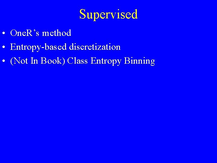
Supervised • One. R’s method • Entropy-based discretization • (Not In Book) Class Entropy Binning

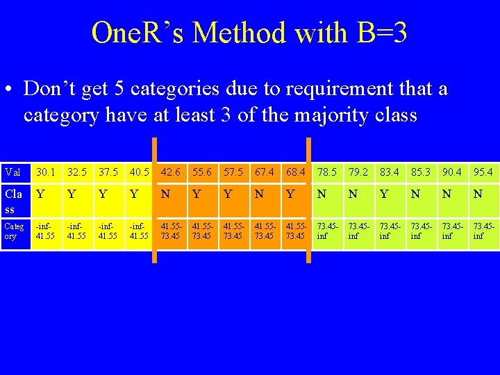
One. R’s Method with B=3 • Don’t get 5 categories due to requirement that a category have at least 3 of the majority class Val 30. 1 32. 5 37. 5 40. 5 42. 6 55. 6 57. 5 67. 4 68. 4 78. 5 79. 2 83. 4 85. 3 90. 4 95. 4 Cla ss Y Y N N Y N N N Categ ory -inf 41. 55 41. 5573. 45 73. 45 inf

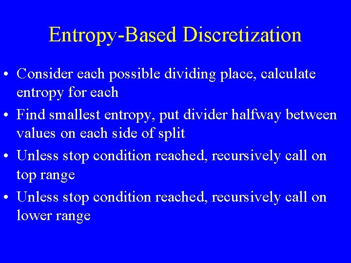
Entropy-Based Discretization • Consider each possible dividing place, calculate entropy for each • Find smallest entropy, put divider halfway between values on each side of split • Unless stop condition reached, recursively call on top range • Unless stop condition reached, recursively call on lower range

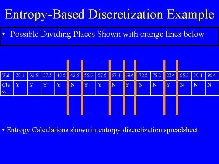
Entropy-Based Discretization Example • Possible Dividing Places Shown with orange lines below Val 30. 1 32. 5 37. 5 40. 5 42. 6 55. 6 57. 5 67. 4 68. 4 78. 5 79. 2 83. 4 85. 3 90. 4 95. 4 Cla ss Y Y N N Y N N N • Entropy Calculations shown in entropy discretization spreadsheet

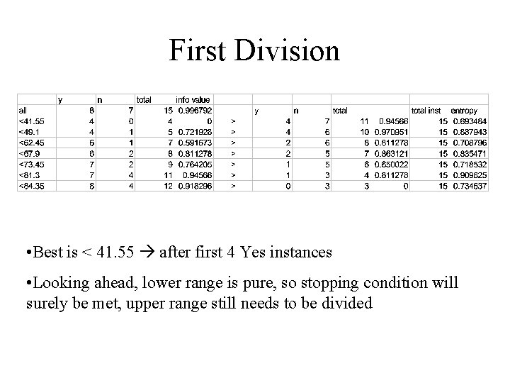
First Division • Best is < 41. 55 after first 4 Yes instances • Looking ahead, lower range is pure, so stopping condition will surely be met, upper range still needs to be divided

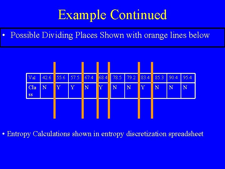
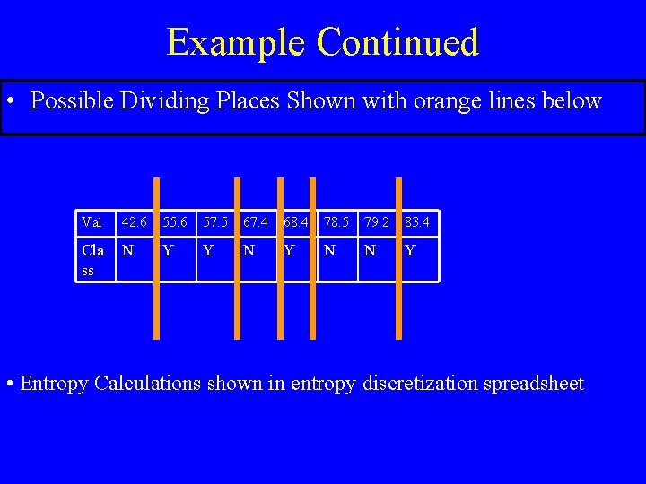
Example Continued • Possible Dividing Places Shown with orange lines below Val 42. 6 55. 6 57. 5 67. 4 68. 4 78. 5 79. 2 83. 4 85. 3 90. 4 95. 4 Cla ss N Y Y N N N • Entropy Calculations shown in entropy discretization spreadsheet

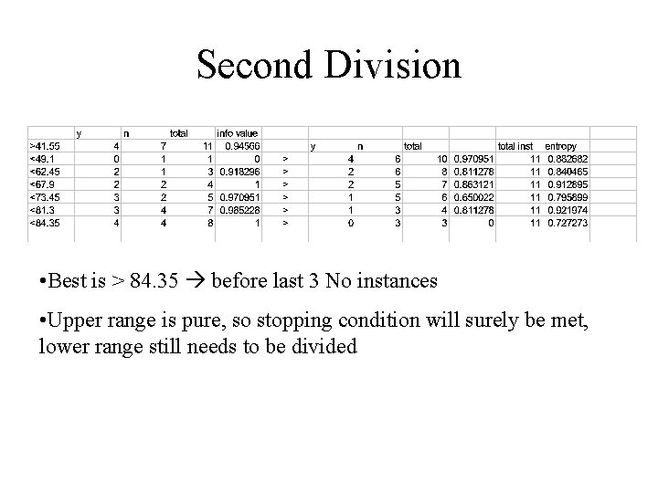
Second Division • Best is > 84. 35 before last 3 No instances • Upper range is pure, so stopping condition will surely be met, lower range still needs to be divided

Example Continued • Possible Dividing Places Shown with orange lines below Val 42. 6 55. 6 57. 5 67. 4 68. 4 78. 5 79. 2 83. 4 Cla ss N Y Y N N Y • Entropy Calculations shown in entropy discretization spreadsheet

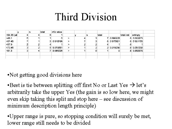
Third Division • Not getting good divisions here • Best is tie between splitting off first No or Last Yes let’s arbitrarily take the upper Yes (the gain is so low here, we might even skip taking this split and stop here – see discussion of minimum description length principle) • Upper range is pure, so stopping condition will surely be met, lower range still needs to be divided

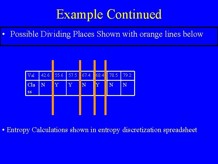
Example Continued • Possible Dividing Places Shown with orange lines below Val 42. 6 55. 6 57. 5 67. 4 68. 4 78. 5 79. 2 Cla ss N Y Y N N • Entropy Calculations shown in entropy discretization spreadsheet

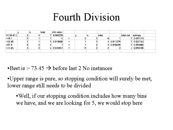
Fourth Division • Best is > 73. 45 before last 2 No instances • Upper range is pure, so stopping condition will surely be met, lower range still needs to be divided • Well, if our stopping condition includes how many bins we have, and we are looking for 5, we would stop here

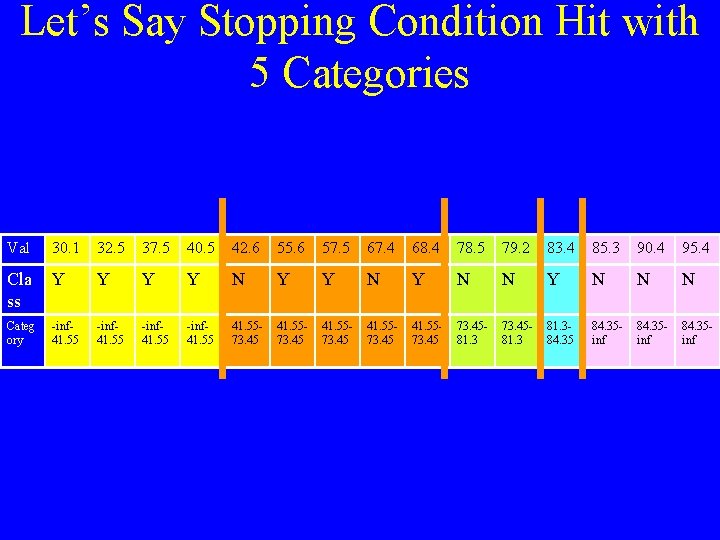
Let’s Say Stopping Condition Hit with 5 Categories Val 30. 1 32. 5 37. 5 40. 5 42. 6 55. 6 57. 5 67. 4 68. 4 78. 5 79. 2 83. 4 85. 3 90. 4 95. 4 Cla ss Y Y N N Y N N N Categ ory -inf 41. 55 41. 5573. 45 73. 4581. 384. 35 inf 84. 35 inf

Combining Multiple Models • When making decisions, it can be valuable to take into account more than one opinion • In data mining, can combine the predictions of multiple models • Generally improves performance • Common methods: bagging, boosting, stacking, error-correcting codes • Negative - Makes “resulting” “model” harder for people to understand

Bagging and Boosting • • Take votes of learned models (For numeric prediction, take average) Bagging – equal votes / averages Boosting – weighted votes / averages – weighted by model’s performance • Another significant difference – – Bagging involves learning separate models (could even be parallel) – Boosting involves iterative generation of models

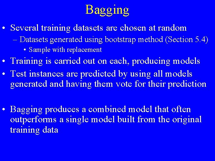
Bagging • Several training datasets are chosen at random – Datasets generated using bootstrap method (Section 5. 4) • Sample with replacement • Training is carried out on each, producing models • Test instances are predicted by using all models generated and having them vote for their prediction • Bagging produces a combined model that often outperforms a single model built from the original training data

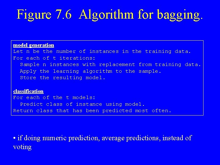
Figure 7. 6 Algorithm for bagging. model generation Let n be the number of instances in the training data. For each of t iterations: Sample n instances with replacement from training data. Apply the learning algorithm to the sample. Store the resulting model. classification For each of the t models: Predict class of instance using model. Return class that has been predicted most often. • if doing numeric prediction, average predictions, instead of voting

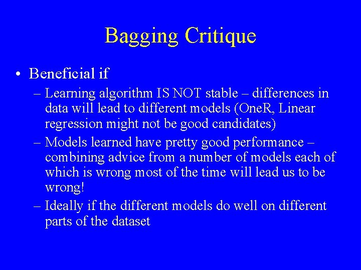
Bagging Critique • Beneficial if – Learning algorithm IS NOT stable – differences in data will lead to different models (One. R, Linear regression might not be good candidates) – Models learned have pretty good performance – combining advice from a number of models each of which is wrong most of the time will lead us to be wrong! – Ideally if the different models do well on different parts of the dataset

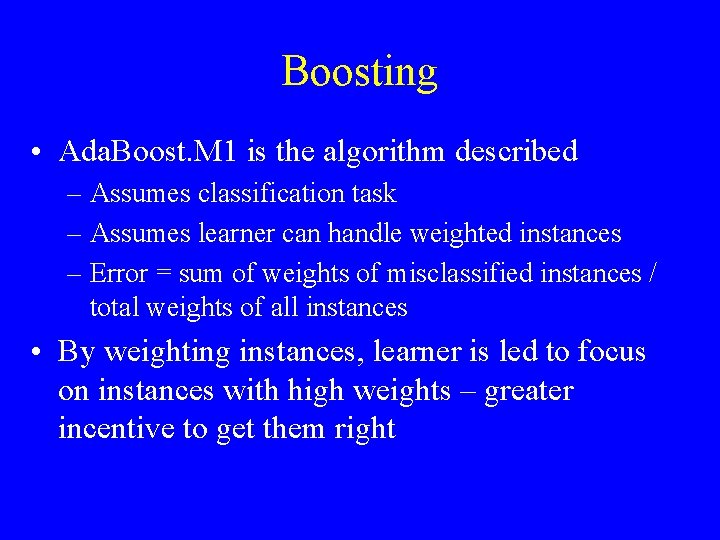
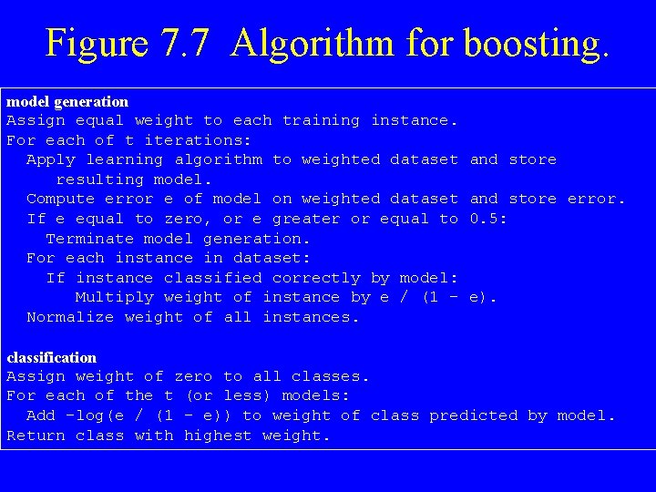
Boosting • Ada. Boost. M 1 is the algorithm described – Assumes classification task – Assumes learner can handle weighted instances – Error = sum of weights of misclassified instances / total weights of all instances • By weighting instances, learner is led to focus on instances with high weights – greater incentive to get them right

Figure 7. 7 Algorithm for boosting. model generation Assign equal weight to each training instance. For each of t iterations: Apply learning algorithm to weighted dataset resulting model. Compute error e of model on weighted dataset If e equal to zero, or e greater or equal to Terminate model generation. For each instance in dataset: If instance classified correctly by model: Multiply weight of instance by e / (1 Normalize weight of all instances. and store error. 0. 5: e). classification Assign weight of zero to all classes. For each of the t (or less) models: Add -log(e / (1 - e)) to weight of class predicted by model. Return class with highest weight.

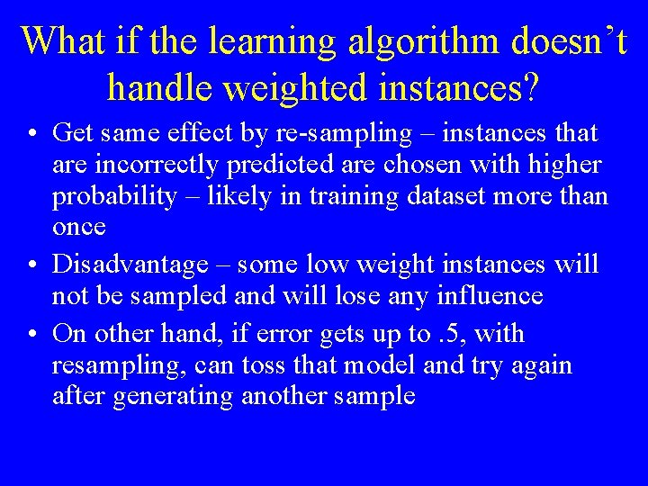
What if the learning algorithm doesn’t handle weighted instances? • Get same effect by re-sampling – instances that are incorrectly predicted are chosen with higher probability – likely in training dataset more than once • Disadvantage – some low weight instances will not be sampled and will lose any influence • On other hand, if error gets up to. 5, with resampling, can toss that model and try again after generating another sample

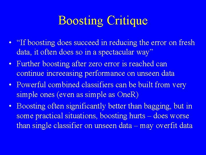
Boosting Critique • “If boosting does succeed in reducing the error on fresh data, it often does so in a spectacular way” • Further boosting after zero error is reached can continue increeasing performance on unseen data • Powerful combined classifiers can be built from very simple ones (even as simple as One. R) • Boosting often significantly better than bagging, but in some practical situations, boosting hurts – does worse than single classifier on unseen data – may overfit data

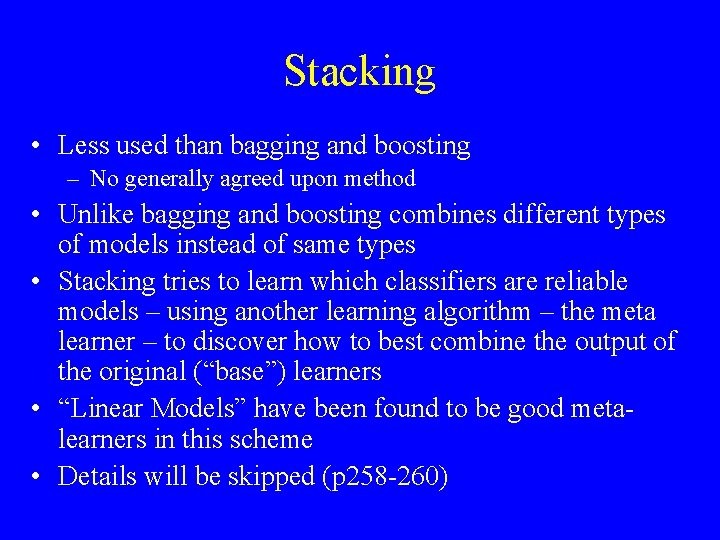
Stacking • Less used than bagging and boosting – No generally agreed upon method • Unlike bagging and boosting combines different types of models instead of same types • Stacking tries to learn which classifiers are reliable models – using another learning algorithm – the meta learner – to discover how to best combine the output of the original (“base”) learners • “Linear Models” have been found to be good metalearners in this scheme • Details will be skipped (p 258 -260)

Error-Correcting Output Codes • SKIP

End Chapter 7