Data Mining Concepts and Techniques Chapter 4 Jiawei

Data Mining: Concepts and Techniques — Chapter 4 — Jiawei Han Department of Computer Science University of Illinois at Urbana-Champaign www. cs. uiuc. edu/~hanj © 2006 Jiawei Han and Micheline Kamber, All rights reserved 6/6/2021 Data Mining: Concepts and Techniques 1

6/6/2021 Data Mining: Concepts and Techniques 2

Chapter 4: Data Cube Computation and Data Generalization n Efficient Computation of Data Cubes n Exploration and Discovery in Multidimensional Databases n Attribute-Oriented Induction ─ An Alternative Data Generalization Method 6/6/2021 Data Mining: Concepts and Techniques 3

Efficient Computation of Data Cubes n Preliminary cube computation tricks (Agarwal et al. ’ 96) n Computing full/iceberg cubes: 3 methodologies n n Top-Down: Multi-Way array aggregation (Zhao, Deshpande & Naughton, SIGMOD’ 97) Bottom-Up: n n H-cubing technique (Han, Pei, Dong & Wang: SIGMOD’ 01) Integrating Top-Down and Bottom-Up: n n Bottom-up computation: BUC (Beyer & Ramarkrishnan, SIGMOD’ 99) Star-cubing algorithm (Xin, Han, Li & Wah: VLDB’ 03) High-dimensional OLAP: A Minimal Cubing Approach (Li, et al. VLDB’ 04) Computing alternative kinds of cubes: n 6/6/2021 Partial cube, closed cube, approximate cube, etc. Data Mining: Concepts and Techniques 4

Preliminary Tricks (Agarwal et al. VLDB’ 96) n n Sorting, hashing, and grouping operations are applied to the dimension attributes in order to reorder and cluster related tuples Aggregates may be computed from previously computed aggregates, rather than from the base fact table n n n 6/6/2021 Smallest-child: computing a cuboid from the smallest, previously computed cuboid Cache-results: caching results of a cuboid from which other cuboids are computed to reduce disk I/Os Amortize-scans: computing as many as possible cuboids at the same time to amortize disk reads Share-sorts: sharing sorting costs cross multiple cuboids when sort-based method is used Share-partitions: sharing the partitioning cost across multiple cuboids when hash-based algorithms are used Data Mining: Concepts and Techniques 5

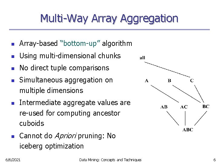
Multi-Way Array Aggregation n Array-based “bottom-up” algorithm n Using multi-dimensional chunks n No direct tuple comparisons n n n Simultaneous aggregation on multiple dimensions Intermediate aggregate values are re-used for computing ancestor cuboids Cannot do Apriori pruning: No iceberg optimization 6/6/2021 Data Mining: Concepts and Techniques 6

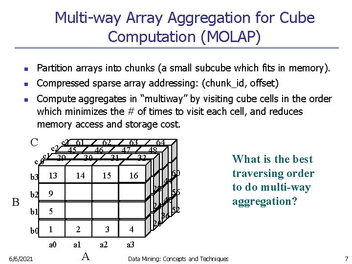
Multi-way Array Aggregation for Cube Computation (MOLAP) n Partition arrays into chunks (a small subcube which fits in memory). n Compressed sparse array addressing: (chunk_id, offset) Compute aggregates in “multiway” by visiting cube cells in the order which minimizes the # of times to visit each cell, and reduces memory access and storage cost. n C c 3 61 62 63 64 c 2 45 46 47 48 c 1 29 30 31 32 c 0 B b 3 B 13 b 2 9 b 1 5 b 0 6/6/2021 14 15 16 1 2 3 4 a 0 a 1 a 2 a 3 A 60 44 28 56 40 24 52 36 20 Data Mining: Concepts and Techniques What is the best traversing order to do multi-way aggregation? 7

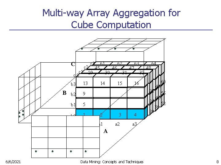
Multi-way Array Aggregation for Cube Computation C c 3 61 62 63 64 c 2 45 46 47 48 c 1 29 30 31 32 c 0 b 3 B b 2 B 13 14 15 16 28 9 24 b 1 5 b 0 1 2 3 4 a 0 a 1 a 2 a 3 20 44 40 36 60 56 52 A 6/6/2021 Data Mining: Concepts and Techniques 8

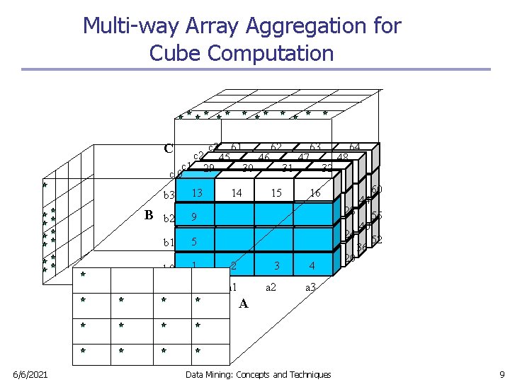
Multi-way Array Aggregation for Cube Computation C c 3 61 62 63 64 c 2 45 46 47 48 c 1 29 30 31 32 c 0 b 3 B b 2 B 13 14 15 16 28 9 24 b 1 5 b 0 1 2 3 4 a 0 a 1 a 2 a 3 20 44 40 36 60 56 52 A 6/6/2021 Data Mining: Concepts and Techniques 9

Multi-Way Array Aggregation for Cube Computation (Cont. ) n Method: the planes should be sorted and computed according to their size in ascending order n n Idea: keep the smallest plane in the main memory, fetch and compute only one chunk at a time for the largest plane Limitation of the method: computing well only for a small number of dimensions n 6/6/2021 If there a large number of dimensions, “top-down” computation and iceberg cube computation methods can be explored Data Mining: Concepts and Techniques 10

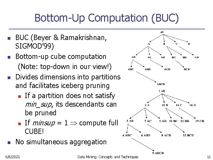
Bottom-Up Computation (BUC) n n BUC (Beyer & Ramakrishnan, SIGMOD’ 99) Bottom-up cube computation (Note: top-down in our view!) Divides dimensions into partitions and facilitates iceberg pruning n If a partition does not satisfy min_sup, its descendants can be pruned n If minsup = 1 Þ compute full CUBE! No simultaneous aggregation 6/6/2021 Data Mining: Concepts and Techniques 11

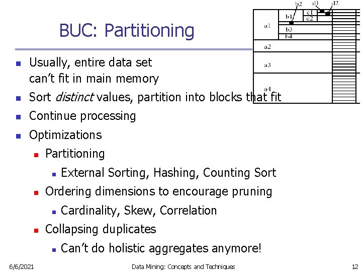
BUC: Partitioning n Usually, entire data set can’t fit in main memory n Sort distinct values, partition into blocks that fit n Continue processing n Optimizations n Partitioning n n Ordering dimensions to encourage pruning n n Cardinality, Skew, Correlation Collapsing duplicates n 6/6/2021 External Sorting, Hashing, Counting Sort Can’t do holistic aggregates anymore! Data Mining: Concepts and Techniques 12

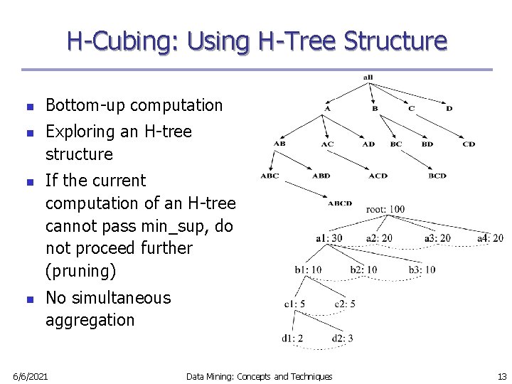
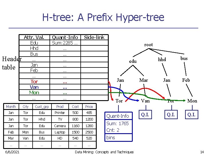
H-Cubing: Using H-Tree Structure n n Bottom-up computation Exploring an H-tree structure If the current computation of an H-tree cannot pass min_sup, do not proceed further (pruning) No simultaneous aggregation 6/6/2021 Data Mining: Concepts and Techniques 13

H-tree: A Prefix Hyper-tree Header table Attr. Val. Edu Hhd Bus … Jan Feb … Tor Van Mon … Quant-Info Sum: 2285 … … … Side-link root Jan Mar Jan Feb Tor Van Tor Mon Quant-Info Q. I. Month City Cust_grp Prod Cost Price Jan Tor Edu Printer 500 485 Jan Tor Hhd TV 800 1200 Jan Tor Edu Camera 1160 1280 Feb Mon Bus Laptop 1500 2500 Sum: 1765 Cnt: 2 Mar Van Edu HD 540 520 bins … … … 6/6/2021 bus hhd edu Data Mining: Concepts and Techniques 14

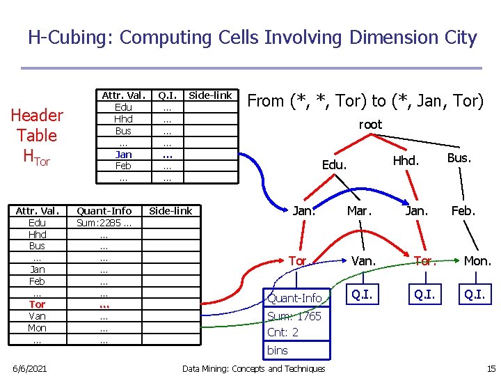
H-Cubing: Computing Cells Involving Dimension City Header Table HTor Attr. Val. Edu Hhd Bus … Jan Feb … Tor Van Mon … 6/6/2021 Attr. Val. Edu Hhd Bus … Jan Feb … Quant-Info Sum: 2285 … … … Q. I. … … … … Side-link From (*, *, Tor) to (*, Jan, Tor) root Hhd. Edu. Jan. Side-link Tor. Quant-Info Mar. Jan. Bus. Feb. Van. Tor. Mon. Q. I. Sum: 1765 Cnt: 2 bins Data Mining: Concepts and Techniques 15

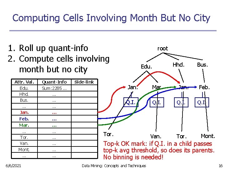
Computing Cells Involving Month But No City 1. Roll up quant-info 2. Compute cells involving month but no city Attr. Val. Edu. Hhd. Bus. … Jan. Feb. Mar. … Tor. Van. Mont. … 6/6/2021 Quant-Info Sum: 2285 … … … Side-link root Hhd. Edu. Jan. Q. I. Tor. Mar. Jan. Q. I. Van. Tor. Bus. Feb. Q. I. Mont. Top-k OK mark: if Q. I. in a child passes top-k avg threshold, so does its parents. No binning is needed! Data Mining: Concepts and Techniques 16

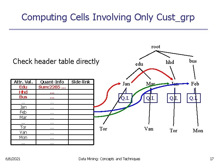
Computing Cells Involving Only Cust_grp root Check header table directly Attr. Val. Edu Hhd Bus … Jan Feb Mar … Tor Van Mon … 6/6/2021 Quant-Info Sum: 2285 … … … hhd edu Side-link bus Jan Mar Jan Feb Q. I. Van Tor Data Mining: Concepts and Techniques Mon 17

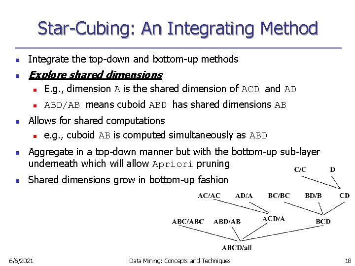
Star-Cubing: An Integrating Method n Integrate the top-down and bottom-up methods n Explore shared dimensions n n E. g. , dimension A is the shared dimension of ACD and AD n ABD/AB means cuboid ABD has shared dimensions AB Allows for shared computations n e. g. , cuboid AB is computed simultaneously as ABD Aggregate in a top-down manner but with the bottom-up sub-layer underneath which will allow Apriori pruning Shared dimensions grow in bottom-up fashion 6/6/2021 Data Mining: Concepts and Techniques 18

Iceberg Pruning in Shared Dimensions n Anti-monotonic property of shared dimensions n n n 6/6/2021 If the measure is anti-monotonic, and if the aggregate value on a shared dimension does not satisfy the iceberg condition, then all the cells extended from this shared dimension cannot satisfy the condition either Intuition: if we can compute the shared dimensions before the actual cuboid, we can use them to do Apriori pruning Problem: how to prune while still aggregate simultaneously on multiple dimensions? Data Mining: Concepts and Techniques 19

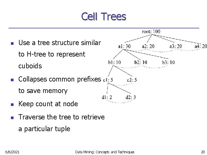
Cell Trees n Use a tree structure similar to H-tree to represent cuboids n Collapses common prefixes to save memory n Keep count at node n Traverse the tree to retrieve a particular tuple 6/6/2021 Data Mining: Concepts and Techniques 20

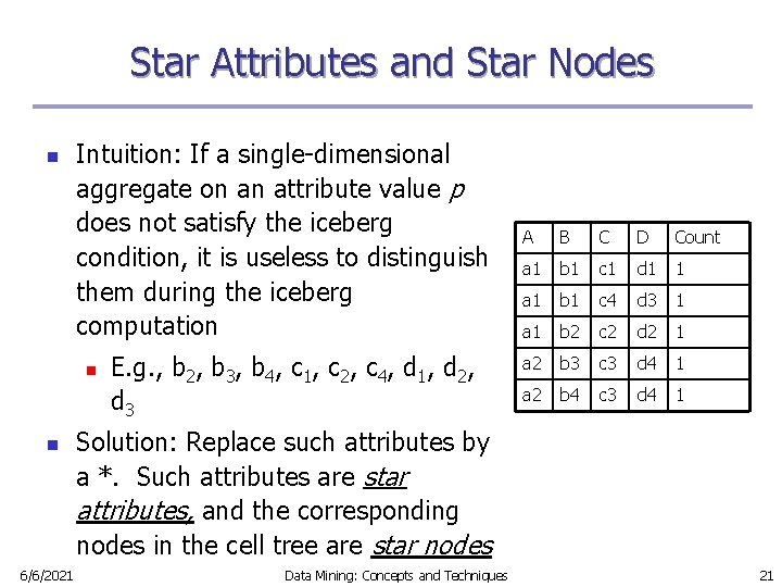
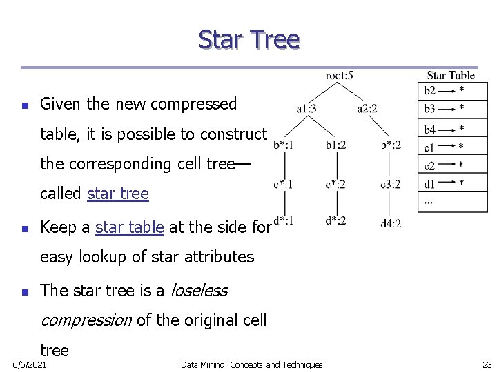
Star Attributes and Star Nodes n Intuition: If a single-dimensional aggregate on an attribute value p does not satisfy the iceberg condition, it is useless to distinguish them during the iceberg computation n n 6/6/2021 E. g. , b 2, b 3, b 4, c 1, c 2, c 4, d 1, d 2, d 3 A B C D Count a 1 b 1 c 1 d 1 1 a 1 b 1 c 4 d 3 1 a 1 b 2 c 2 d 2 1 a 2 b 3 c 3 d 4 1 a 2 b 4 c 3 d 4 1 Solution: Replace such attributes by a *. Such attributes are star attributes, and the corresponding nodes in the cell tree are star nodes Data Mining: Concepts and Techniques 21

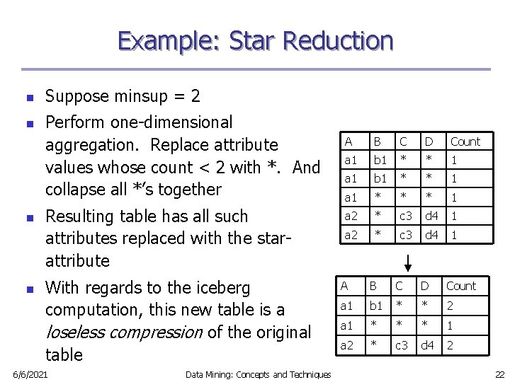
Example: Star Reduction n n Suppose minsup = 2 Perform one-dimensional aggregation. Replace attribute values whose count < 2 with *. And collapse all *’s together Resulting table has all such attributes replaced with the starattribute With regards to the iceberg computation, this new table is a loseless compression of the original table 6/6/2021 Data Mining: Concepts and Techniques A B C D Count a 1 b 1 * * 1 a 1 * * * 1 a 2 * c 3 d 4 1 A B C D Count a 1 b 1 * * 2 a 1 * * * 1 a 2 * c 3 d 4 2 22

Star Tree n Given the new compressed table, it is possible to construct the corresponding cell tree— called star tree n Keep a star table at the side for easy lookup of star attributes n The star tree is a loseless compression of the original cell tree 6/6/2021 Data Mining: Concepts and Techniques 23

Star-Cubing Algorithm—DFS on Lattice Tree 6/6/2021 Data Mining: Concepts and Techniques 24

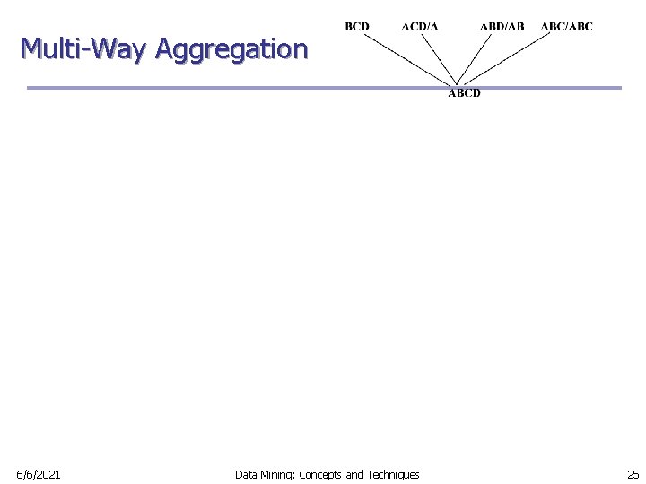
Multi-Way Aggregation 6/6/2021 Data Mining: Concepts and Techniques 25

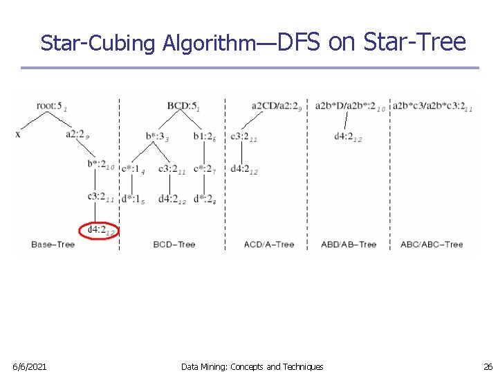
Star-Cubing Algorithm—DFS on Star-Tree 6/6/2021 Data Mining: Concepts and Techniques 26

Multi-Way Star-Tree Aggregation n Start depth-first search at the root of the base star tree n At each new node in the DFS, create corresponding star tree that are descendents of the current tree according to the integrated traversal ordering n E. g. , in the base tree, when DFS reaches a 1, the ACD/A tree is created n n When DFS reaches b*, the ABD/AD tree is created The counts in the base tree are carried over to the new trees 6/6/2021 Data Mining: Concepts and Techniques 27

Multi-Way Aggregation (2) n n n When DFS reaches a leaf node (e. g. , d*), start backtracking On every backtracking branch, the count in the corresponding trees are output, the tree is destroyed, and the node in the base tree is destroyed Example n When traversing from d* back to c*, the a 1 b*c*/a 1 b*c* tree is output and destroyed n n 6/6/2021 When traversing from c* back to b*, the a 1 b*D/a 1 b* tree is output and destroyed When at b*, jump to b 1 and repeat similar process Data Mining: Concepts and Techniques 28

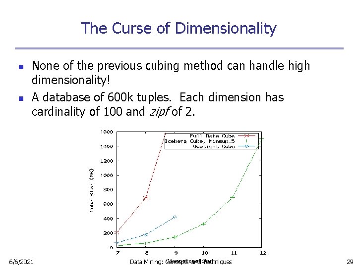
The Curse of Dimensionality n n None of the previous cubing method can handle high dimensionality! A database of 600 k tuples. Each dimension has cardinality of 100 and zipf of 2. 6/6/2021 Data Mining: Concepts and Techniques 29

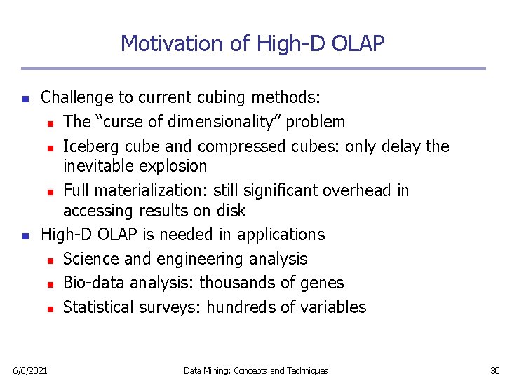
Motivation of High-D OLAP n n Challenge to current cubing methods: n The “curse of dimensionality’’ problem n Iceberg cube and compressed cubes: only delay the inevitable explosion n Full materialization: still significant overhead in accessing results on disk High-D OLAP is needed in applications n Science and engineering analysis n Bio-data analysis: thousands of genes n Statistical surveys: hundreds of variables 6/6/2021 Data Mining: Concepts and Techniques 30

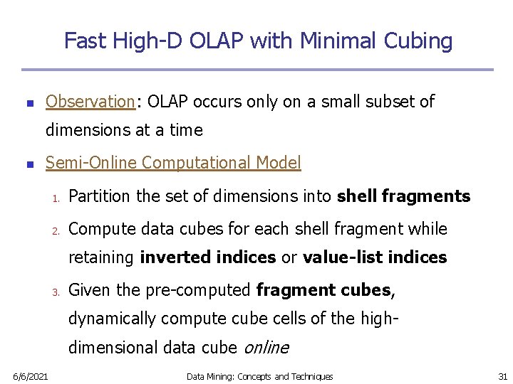
Fast High-D OLAP with Minimal Cubing n Observation: OLAP occurs only on a small subset of dimensions at a time n Semi-Online Computational Model 1. Partition the set of dimensions into shell fragments 2. Compute data cubes for each shell fragment while retaining inverted indices or value-list indices 3. Given the pre-computed fragment cubes, dynamically compute cube cells of the highdimensional data cube online 6/6/2021 Data Mining: Concepts and Techniques 31

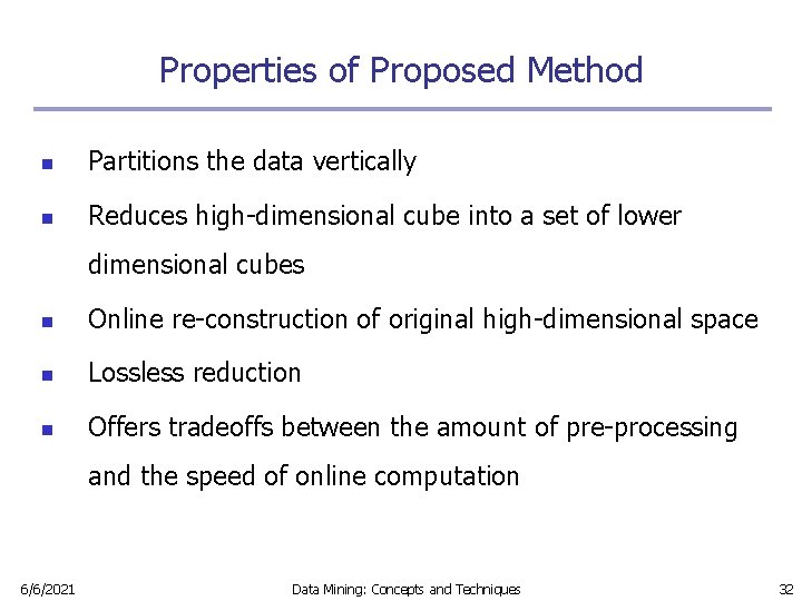
Properties of Proposed Method n Partitions the data vertically n Reduces high-dimensional cube into a set of lower dimensional cubes n Online re-construction of original high-dimensional space n Lossless reduction n Offers tradeoffs between the amount of pre-processing and the speed of online computation 6/6/2021 Data Mining: Concepts and Techniques 32

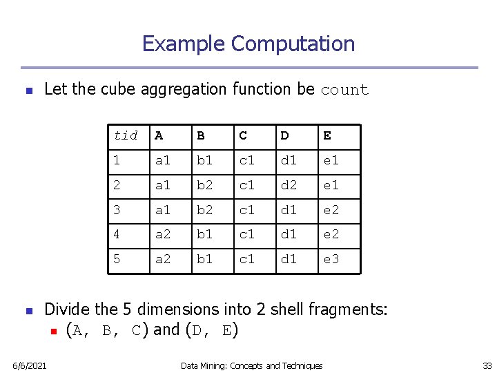
Example Computation n n Let the cube aggregation function be count tid A B C D E 1 a 1 b 1 c 1 d 1 e 1 2 a 1 b 2 c 1 d 2 e 1 3 a 1 b 2 c 1 d 1 e 2 4 a 2 b 1 c 1 d 1 e 2 5 a 2 b 1 c 1 d 1 e 3 Divide the 5 dimensions into 2 shell fragments: n (A, B, C) and (D, E) 6/6/2021 Data Mining: Concepts and Techniques 33

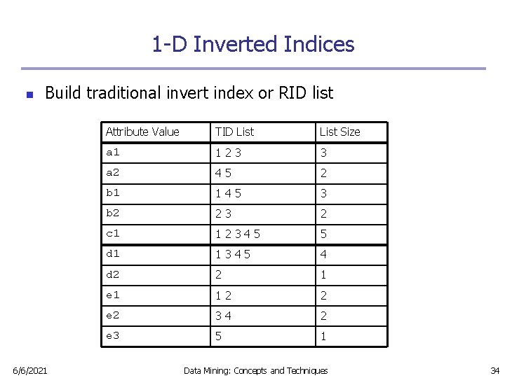
1 -D Inverted Indices n Build traditional invert index or RID list 6/6/2021 Attribute Value TID List Size a 1 123 3 a 2 45 2 b 1 145 3 b 2 23 2 c 1 12345 5 d 1 1345 4 d 2 2 1 e 1 12 2 e 2 34 2 e 3 5 1 Data Mining: Concepts and Techniques 34

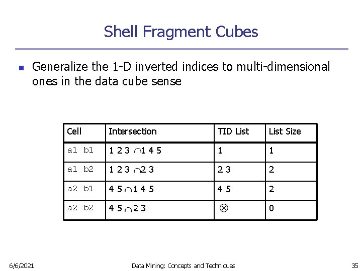
Shell Fragment Cubes n Generalize the 1 -D inverted indices to multi-dimensional ones in the data cube sense 6/6/2021 Cell Intersection TID List Size a 1 b 1 123 145 1 1 a 1 b 2 123 23 23 2 a 2 b 1 45 145 45 2 a 2 b 2 45 23 Data Mining: Concepts and Techniques 0 35

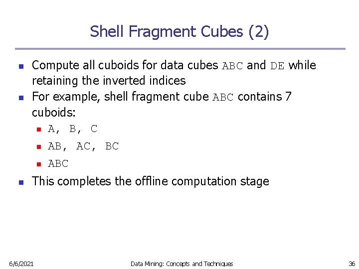
Shell Fragment Cubes (2) n n n Compute all cuboids for data cubes ABC and DE while retaining the inverted indices For example, shell fragment cube ABC contains 7 cuboids: n A, B, C n AB, AC, BC n ABC This completes the offline computation stage 6/6/2021 Data Mining: Concepts and Techniques 36

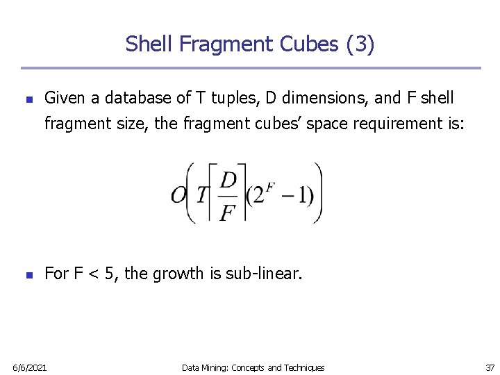
Shell Fragment Cubes (3) n Given a database of T tuples, D dimensions, and F shell fragment size, the fragment cubes’ space requirement is: n For F < 5, the growth is sub-linear. 6/6/2021 Data Mining: Concepts and Techniques 37

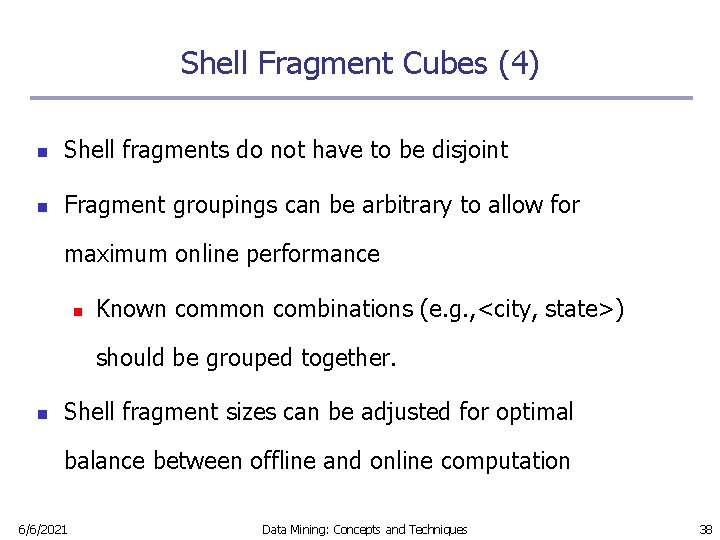
Shell Fragment Cubes (4) n Shell fragments do not have to be disjoint n Fragment groupings can be arbitrary to allow for maximum online performance n Known common combinations (e. g. , <city, state>) should be grouped together. n Shell fragment sizes can be adjusted for optimal balance between offline and online computation 6/6/2021 Data Mining: Concepts and Techniques 38

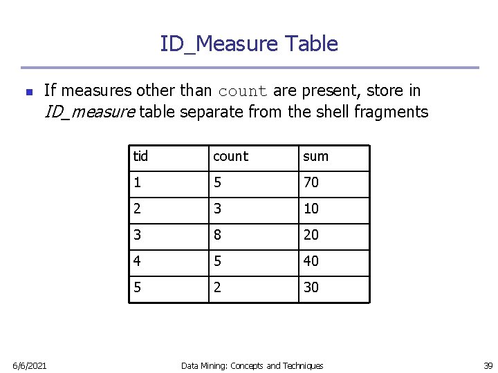
ID_Measure Table n If measures other than count are present, store in ID_measure table separate from the shell fragments 6/6/2021 tid count sum 1 5 70 2 3 10 3 8 20 4 5 40 5 2 30 Data Mining: Concepts and Techniques 39

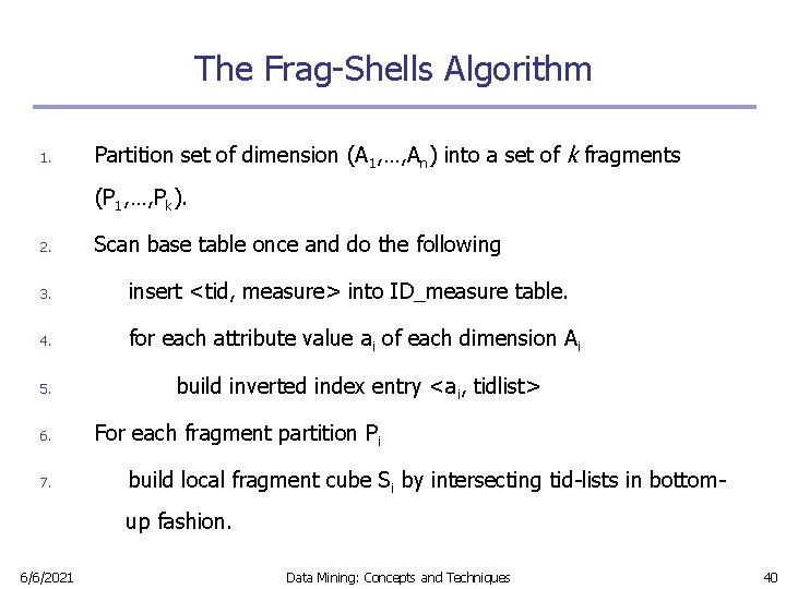
The Frag-Shells Algorithm 1. Partition set of dimension (A 1, …, An) into a set of k fragments (P 1, …, Pk). 2. Scan base table once and do the following 3. insert <tid, measure> into ID_measure table. 4. for each attribute value ai of each dimension Ai 5. build inverted index entry <ai, tidlist> 6. 7. For each fragment partition Pi build local fragment cube Si by intersecting tid-lists in bottomup fashion. 6/6/2021 Data Mining: Concepts and Techniques 40

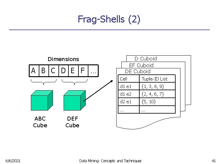
Frag-Shells (2) Dimensions D Cuboid EF Cuboid DE Cuboid A B C D E F … ABC Cube 6/6/2021 Cell Tuple-ID List d 1 e 1 {1, 3, 8, 9} d 1 e 2 {2, 4, 6, 7} d 2 e 1 {5, 10} … … DEF Cube Data Mining: Concepts and Techniques 41

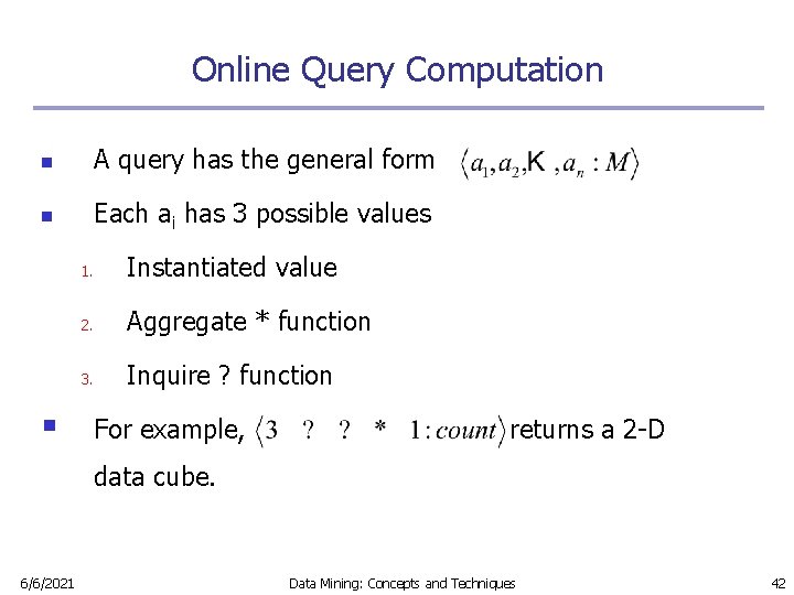
Online Query Computation n A query has the general form n Each ai has 3 possible values § 1. Instantiated value 2. Aggregate * function 3. Inquire ? function For example, returns a 2 -D data cube. 6/6/2021 Data Mining: Concepts and Techniques 42

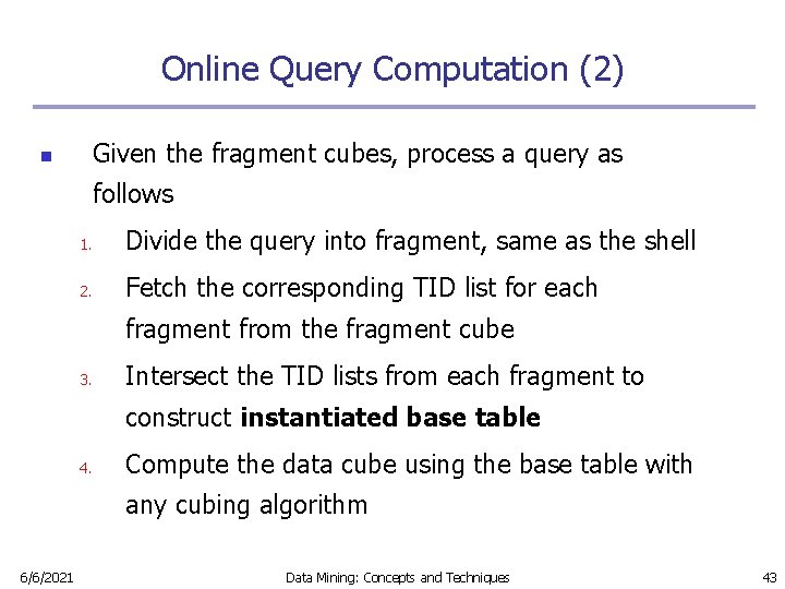
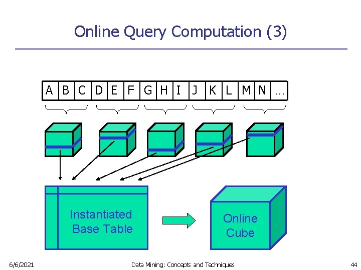
Online Query Computation (2) Given the fragment cubes, process a query as n follows 1. Divide the query into fragment, same as the shell 2. Fetch the corresponding TID list for each fragment from the fragment cube 3. Intersect the TID lists from each fragment to construct instantiated base table 4. Compute the data cube using the base table with any cubing algorithm 6/6/2021 Data Mining: Concepts and Techniques 43

Online Query Computation (3) A B C D E F G H I J K L M N … Instantiated Base Table 6/6/2021 Online Cube Data Mining: Concepts and Techniques 44

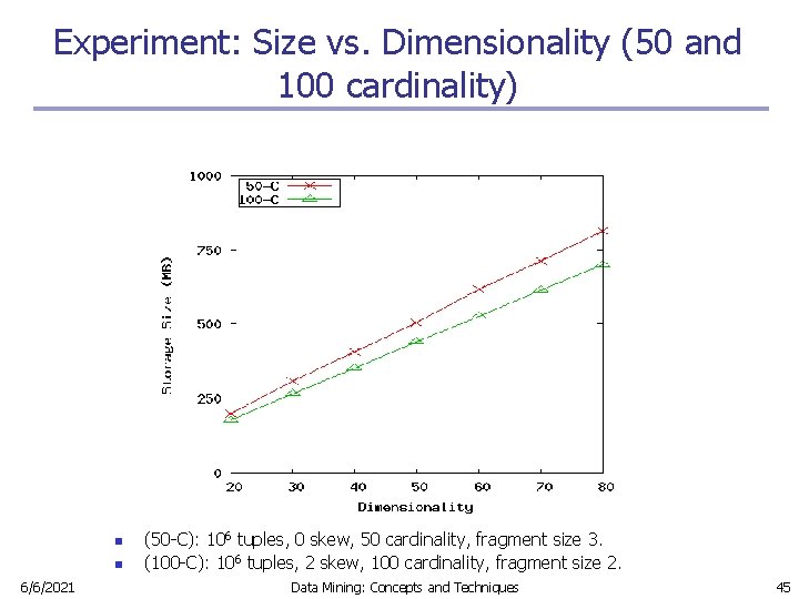
Experiment: Size vs. Dimensionality (50 and 100 cardinality) n n 6/6/2021 (50 -C): 106 tuples, 0 skew, 50 cardinality, fragment size 3. (100 -C): 106 tuples, 2 skew, 100 cardinality, fragment size 2. Data Mining: Concepts and Techniques 45

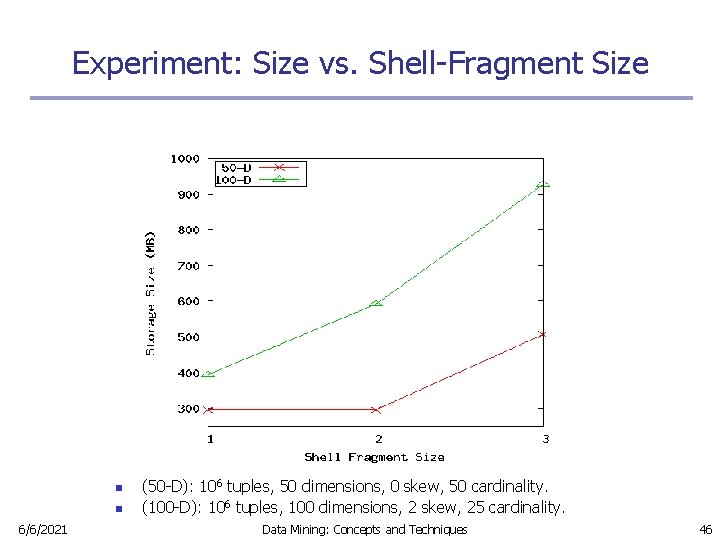
Experiment: Size vs. Shell-Fragment Size n n 6/6/2021 (50 -D): 106 tuples, 50 dimensions, 0 skew, 50 cardinality. (100 -D): 106 tuples, 100 dimensions, 2 skew, 25 cardinality. Data Mining: Concepts and Techniques 46

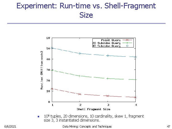
Experiment: Run-time vs. Shell-Fragment Size n 6/6/2021 106 tuples, 20 dimensions, 10 cardinality, skew 1, fragment size 3, 3 instantiated dimensions. Data Mining: Concepts and Techniques 47

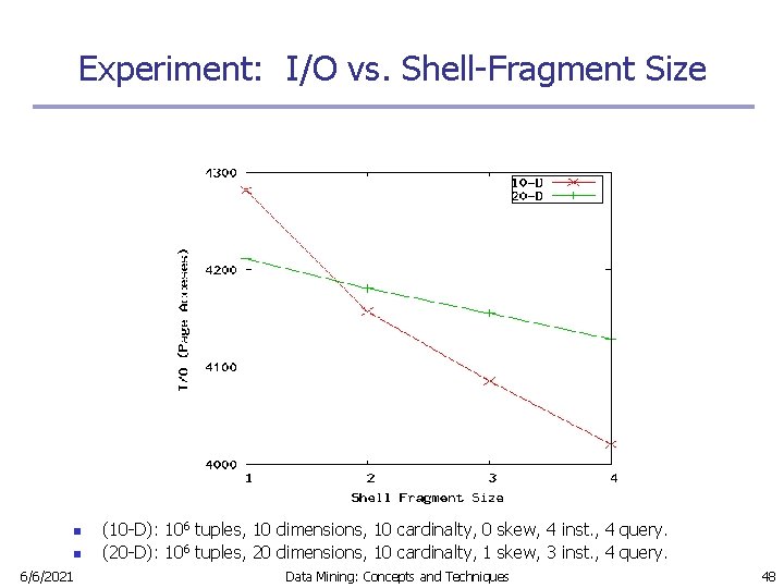
Experiment: I/O vs. Shell-Fragment Size n n 6/6/2021 (10 -D): 106 tuples, 10 dimensions, 10 cardinalty, 0 skew, 4 inst. , 4 query. (20 -D): 106 tuples, 20 dimensions, 10 cardinalty, 1 skew, 3 inst. , 4 query. Data Mining: Concepts and Techniques 48

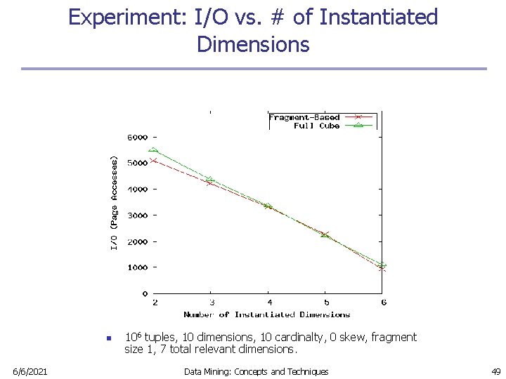
Experiment: I/O vs. # of Instantiated Dimensions n 6/6/2021 106 tuples, 10 dimensions, 10 cardinalty, 0 skew, fragment size 1, 7 total relevant dimensions. Data Mining: Concepts and Techniques 49

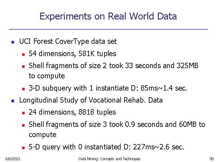
Experiments on Real World Data n UCI Forest Cover. Type data set n n 54 dimensions, 581 K tuples Shell fragments of size 2 took 33 seconds and 325 MB to compute 3 -D subquery with 1 instantiate D: 85 ms~1. 4 sec. Longitudinal Study of Vocational Rehab. Data n n n 6/6/2021 24 dimensions, 8818 tuples Shell fragments of size 3 took 0. 9 seconds and 60 MB to compute 5 -D query with 0 instantiated D: 227 ms~2. 6 sec. Data Mining: Concepts and Techniques 50

Comparisons to Related Work n [Harinarayan 96] computes low-dimensional cuboids by further aggregation of high-dimensional cuboids. Opposite of our method’s direction. n Inverted indexing structures [Witten 99] focus on single dimensional data or multi-dimensional data with no aggregation. n Tree-stripping [Berchtold 00] uses similar vertical partitioning of database but no aggregation. 6/6/2021 Data Mining: Concepts and Techniques 51

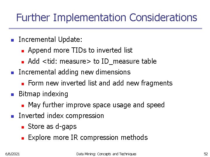
Further Implementation Considerations n n Incremental Update: n Append more TIDs to inverted list n Add <tid: measure> to ID_measure table Incremental adding new dimensions n n Bitmap indexing n n Form new inverted list and add new fragments May further improve space usage and speed Inverted index compression 6/6/2021 n Store as d-gaps n Explore more IR compression methods Data Mining: Concepts and Techniques 52

Chapter 4: Data Cube Computation and Data Generalization n Efficient Computation of Data Cubes n Exploration and Discovery in Multidimensional Databases n Attribute-Oriented Induction ─ An Alternative Data Generalization Method 6/6/2021 Data Mining: Concepts and Techniques 53

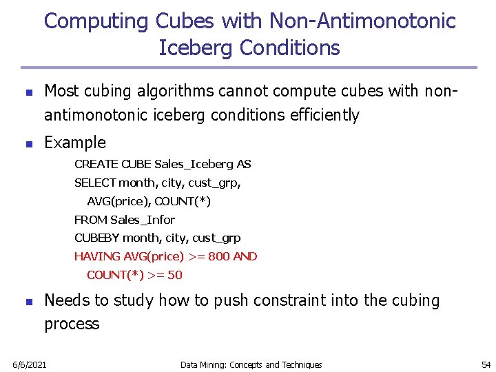
Computing Cubes with Non-Antimonotonic Iceberg Conditions n n Most cubing algorithms cannot compute cubes with nonantimonotonic iceberg conditions efficiently Example CREATE CUBE Sales_Iceberg AS SELECT month, city, cust_grp, AVG(price), COUNT(*) FROM Sales_Infor CUBEBY month, city, cust_grp HAVING AVG(price) >= 800 AND COUNT(*) >= 50 n Needs to study how to push constraint into the cubing process 6/6/2021 Data Mining: Concepts and Techniques 54

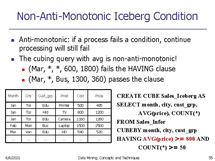
Non-Anti-Monotonic Iceberg Condition n n Anti-monotonic: if a process fails a condition, continue processing will still fail The cubing query with avg is non-anti-monotonic! n (Mar, *, *, 600, 1800) fails the HAVING clause n (Mar, *, Bus, 1300, 360) passes the clause Month City Cust_grp Prod Cost Price Jan Tor Edu Printer 500 485 Jan Tor Hld TV 800 1200 Jan Tor Edu Camera 1160 1280 Feb Mon Bus Laptop 1500 2500 Mar Van Edu HD 540 520 … … … 6/6/2021 CREATE CUBE Sales_Iceberg AS SELECT month, city, cust_grp, AVG(price), COUNT(*) FROM Sales_Infor CUBEBY month, city, cust_grp HAVING AVG(price) >= 800 AND COUNT(*) >= 50 Data Mining: Concepts and Techniques 55

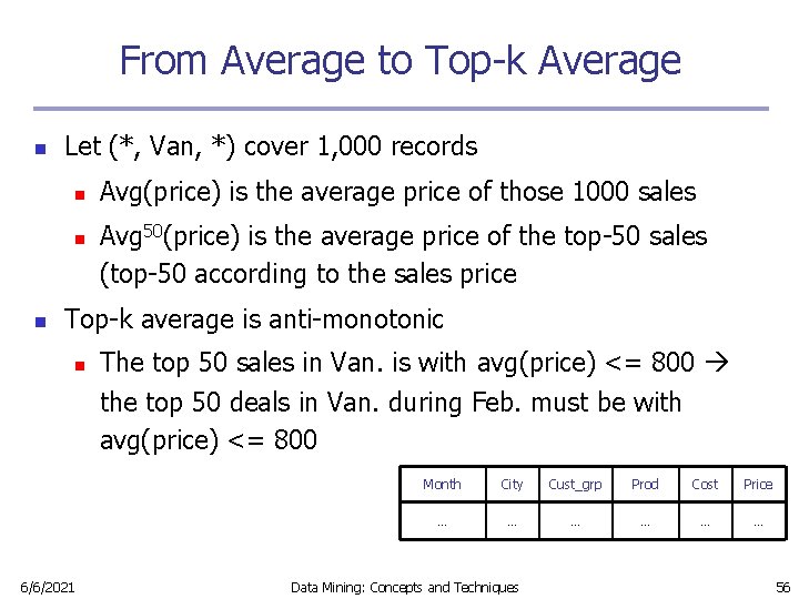
From Average to Top-k Average n Let (*, Van, *) cover 1, 000 records n n n Avg(price) is the average price of those 1000 sales Avg 50(price) is the average price of the top-50 sales (top-50 according to the sales price Top-k average is anti-monotonic n 6/6/2021 The top 50 sales in Van. is with avg(price) <= 800 the top 50 deals in Van. during Feb. must be with avg(price) <= 800 Month City Cust_grp Prod Cost Price … … … Data Mining: Concepts and Techniques 56

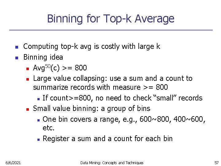
Binning for Top-k Average n n 6/6/2021 Computing top-k avg is costly with large k Binning idea 50 n Avg (c) >= 800 n Large value collapsing: use a sum and a count to summarize records with measure >= 800 n If count>=800, no need to check “small” records n Small value binning: a group of bins n One bin covers a range, e. g. , 600~800, 400~600, etc. n Register a sum and a count for each bin Data Mining: Concepts and Techniques 57

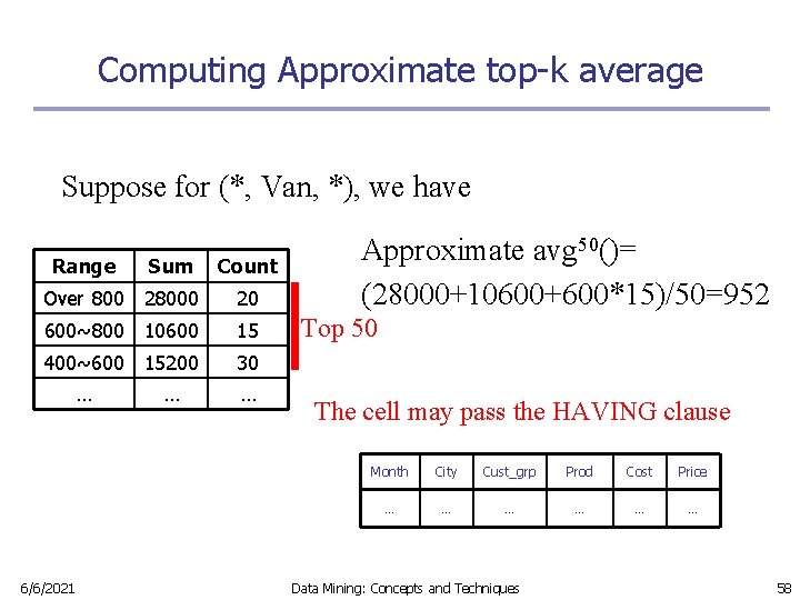
Computing Approximate top-k average Suppose for (*, Van, *), we have Range Sum Count Over 800 28000 20 600~800 10600 15 400~600 15200 30 … … … 6/6/2021 Approximate avg 50()= (28000+10600+600*15)/50=952 Top 50 The cell may pass the HAVING clause Month City Cust_grp Prod Cost Price … … … Data Mining: Concepts and Techniques 58

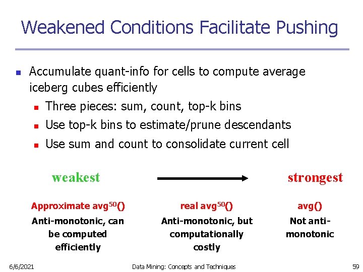
Weakened Conditions Facilitate Pushing n Accumulate quant-info for cells to compute average iceberg cubes efficiently n Three pieces: sum, count, top-k bins n Use top-k bins to estimate/prune descendants n Use sum and count to consolidate current cell weakest strongest Approximate avg 50() real avg 50() avg() Anti-monotonic, can be computed efficiently Anti-monotonic, but computationally costly Not antimonotonic 6/6/2021 Data Mining: Concepts and Techniques 59

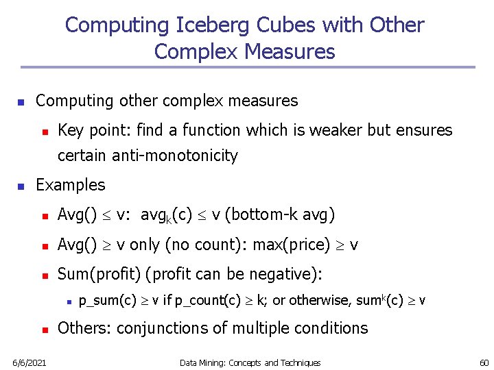
Computing Iceberg Cubes with Other Complex Measures n Computing other complex measures n Key point: find a function which is weaker but ensures certain anti-monotonicity n Examples n Avg() v: avgk(c) v (bottom-k avg) n Avg() v only (no count): max(price) v n Sum(profit) (profit can be negative): n n 6/6/2021 p_sum(c) v if p_count(c) k; or otherwise, sumk(c) v Others: conjunctions of multiple conditions Data Mining: Concepts and Techniques 60

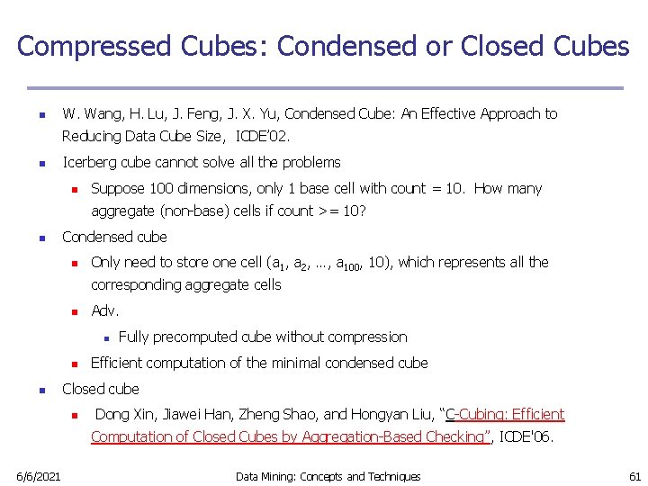
Compressed Cubes: Condensed or Closed Cubes n W. Wang, H. Lu, J. Feng, J. X. Yu, Condensed Cube: An Effective Approach to Reducing Data Cube Size, ICDE’ 02. n Icerberg cube cannot solve all the problems n Suppose 100 dimensions, only 1 base cell with count = 10. How many aggregate (non-base) cells if count >= 10? n Condensed cube n Only need to store one cell (a 1, a 2, …, a 100, 10), which represents all the corresponding aggregate cells n Adv. n n n Fully precomputed cube without compression Efficient computation of the minimal condensed cube Closed cube n Dong Xin, Jiawei Han, Zheng Shao, and Hongyan Liu, “C-Cubing: Efficient Computation of Closed Cubes by Aggregation-Based Checking”, ICDE'06. 6/6/2021 Data Mining: Concepts and Techniques 61

Chapter 4: Data Cube Computation and Data Generalization n Efficient Computation of Data Cubes n Exploration and Discovery in Multidimensional Databases n Attribute-Oriented Induction ─ An Alternative Data Generalization Method 6/6/2021 Data Mining: Concepts and Techniques 62

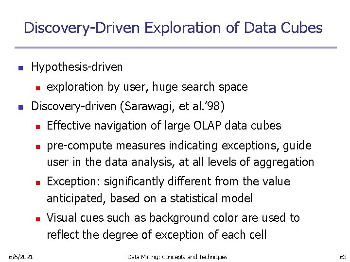
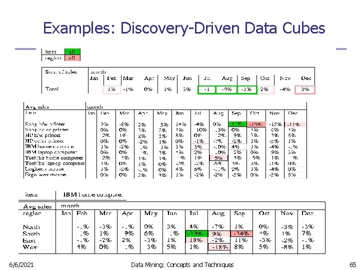
Discovery-Driven Exploration of Data Cubes n Hypothesis-driven n n exploration by user, huge search space Discovery-driven (Sarawagi, et al. ’ 98) n n 6/6/2021 Effective navigation of large OLAP data cubes pre-compute measures indicating exceptions, guide user in the data analysis, at all levels of aggregation Exception: significantly different from the value anticipated, based on a statistical model Visual cues such as background color are used to reflect the degree of exception of each cell Data Mining: Concepts and Techniques 63

Kinds of Exceptions and their Computation n Parameters n n n Self. Exp: surprise of cell relative to other cells at same level of aggregation n In. Exp: surprise beneath the cell n Path. Exp: surprise beneath cell for each drill-down path Computation of exception indicator (modeling fitting and computing Self. Exp, In. Exp, and Path. Exp values) can be overlapped with cube construction Exception themselves can be stored, indexed and retrieved like precomputed aggregates 6/6/2021 Data Mining: Concepts and Techniques 64

Examples: Discovery-Driven Data Cubes 6/6/2021 Data Mining: Concepts and Techniques 65

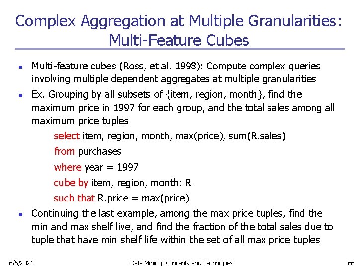
Complex Aggregation at Multiple Granularities: Multi-Feature Cubes n n Multi-feature cubes (Ross, et al. 1998): Compute complex queries involving multiple dependent aggregates at multiple granularities Ex. Grouping by all subsets of {item, region, month}, find the maximum price in 1997 for each group, and the total sales among all maximum price tuples select item, region, month, max(price), sum(R. sales) from purchases where year = 1997 cube by item, region, month: R such that R. price = max(price) n Continuing the last example, among the max price tuples, find the min and max shelf live, and find the fraction of the total sales due to tuple that have min shelf life within the set of all max price tuples 6/6/2021 Data Mining: Concepts and Techniques 66

Cube-Gradient (Cubegrade) n Analysis of changes of sophisticated measures in multidimensional spaces n n n Query: changes of average house price in Vancouver in ‘ 00 comparing against ’ 99 Answer: Apts in West went down 20%, houses in Metrotown went up 10% Cubegrade problem by Imielinski et al. 6/6/2021 n Changes in dimensions changes in measures n Drill-down, roll-up, and mutation Data Mining: Concepts and Techniques 67

From Cubegrade to Multi-dimensional Constrained Gradients in Data Cubes n Significantly more expressive than association rules n n Capture trends in user-specified measures Serious challenges n n n 6/6/2021 Many trivial cells in a cube “significance constraint” to prune trivial cells Numerate pairs of cells “probe constraint” to select a subset of cells to examine Only interesting changes wanted “gradient constraint” to capture significant changes Data Mining: Concepts and Techniques 68

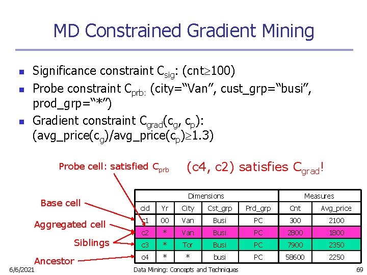
MD Constrained Gradient Mining n n n Significance constraint Csig: (cnt 100) Probe constraint Cprb: (city=“Van”, cust_grp=“busi”, prod_grp=“*”) Gradient constraint Cgrad(cg, cp): (avg_price(cg)/avg_price(cp) 1. 3) Probe cell: satisfied Cprb Base cell Aggregated cell Siblings Ancestor 6/6/2021 (c 4, c 2) satisfies Cgrad! Dimensions Measures cid Yr City Cst_grp Prd_grp Cnt Avg_price c 1 00 Van Busi PC 300 2100 c 2 * Van Busi PC 2800 1800 c 3 * Tor Busi PC 7900 2350 c 4 * * busi PC 58600 2250 Data Mining: Concepts and Techniques 69

Efficient Computing Cube-gradients n Compute probe cells using Csig and Cprb n n The set of probe cells P is often very small Use probe P and constraints to find gradients n Pushing selection deeply n Set-oriented processing for probe cells n Iceberg growing from low to high dimensionalities n Dynamic pruning probe cells during growth n Incorporating efficient iceberg cubing method 6/6/2021 Data Mining: Concepts and Techniques 70

Chapter 4: Data Cube Computation and Data Generalization n Efficient Computation of Data Cubes n Exploration and Discovery in Multidimensional Databases n Attribute-Oriented Induction ─ An Alternative Data Generalization Method 6/6/2021 Data Mining: Concepts and Techniques 71

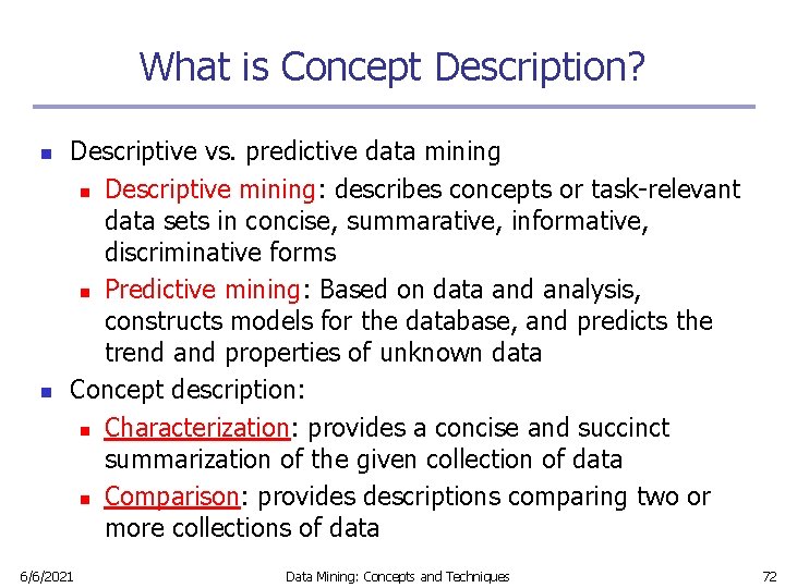
What is Concept Description? n n Descriptive vs. predictive data mining n Descriptive mining: describes concepts or task-relevant data sets in concise, summarative, informative, discriminative forms n Predictive mining: Based on data and analysis, constructs models for the database, and predicts the trend and properties of unknown data Concept description: n Characterization: provides a concise and succinct summarization of the given collection of data n Comparison: provides descriptions comparing two or more collections of data 6/6/2021 Data Mining: Concepts and Techniques 72

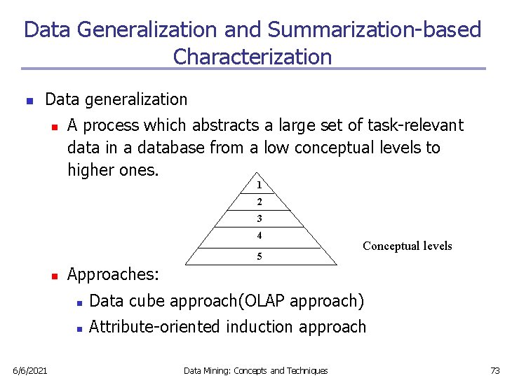
Data Generalization and Summarization-based Characterization n Data generalization n A process which abstracts a large set of task-relevant data in a database from a low conceptual levels to higher ones. 1 2 3 4 5 n 6/6/2021 Conceptual levels Approaches: n Data cube approach(OLAP approach) n Attribute-oriented induction approach Data Mining: Concepts and Techniques 73

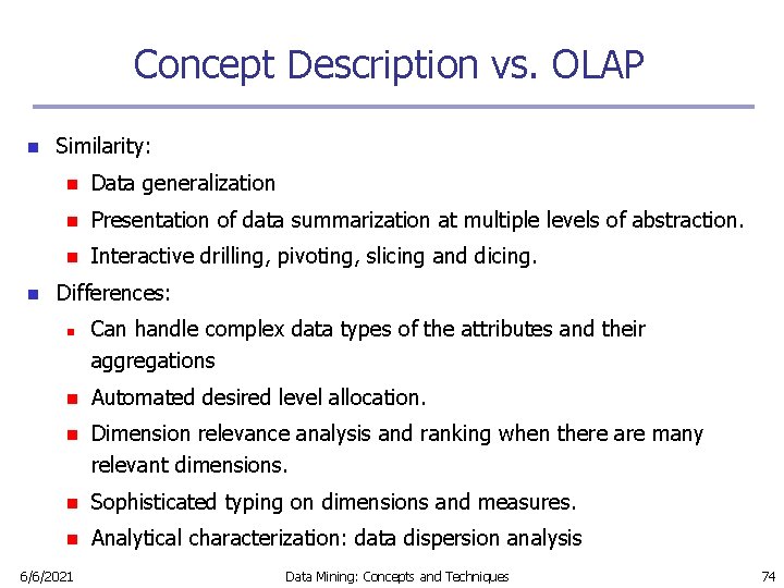
Concept Description vs. OLAP n n Similarity: n Data generalization n Presentation of data summarization at multiple levels of abstraction. n Interactive drilling, pivoting, slicing and dicing. Differences: n Can handle complex data types of the attributes and their aggregations n Automated desired level allocation. n Dimension relevance analysis and ranking when there are many relevant dimensions. n Sophisticated typing on dimensions and measures. n Analytical characterization: data dispersion analysis 6/6/2021 Data Mining: Concepts and Techniques 74

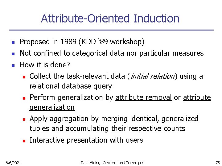
Attribute-Oriented Induction n Proposed in 1989 (KDD ‘ 89 workshop) n Not confined to categorical data nor particular measures n How it is done? n n 6/6/2021 Collect the task-relevant data (initial relation) using a relational database query Perform generalization by attribute removal or attribute generalization Apply aggregation by merging identical, generalized tuples and accumulating their respective counts Interactive presentation with users Data Mining: Concepts and Techniques 75

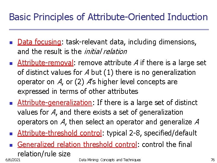
Basic Principles of Attribute-Oriented Induction n n Data focusing: task-relevant data, including dimensions, and the result is the initial relation Attribute-removal: remove attribute A if there is a large set of distinct values for A but (1) there is no generalization operator on A, or (2) A’s higher level concepts are expressed in terms of other attributes Attribute-generalization: If there is a large set of distinct values for A, and there exists a set of generalization operators on A, then select an operator and generalize A Attribute-threshold control: typical 2 -8, specified/default Generalized relation threshold control: control the final relation/rule size 6/6/2021 Data Mining: Concepts and Techniques 76

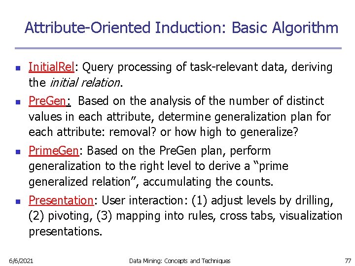
Attribute-Oriented Induction: Basic Algorithm n n Initial. Rel: Query processing of task-relevant data, deriving the initial relation. Pre. Gen: Based on the analysis of the number of distinct values in each attribute, determine generalization plan for each attribute: removal? or how high to generalize? Prime. Gen: Based on the Pre. Gen plan, perform generalization to the right level to derive a “prime generalized relation”, accumulating the counts. Presentation: User interaction: (1) adjust levels by drilling, (2) pivoting, (3) mapping into rules, cross tabs, visualization presentations. 6/6/2021 Data Mining: Concepts and Techniques 77

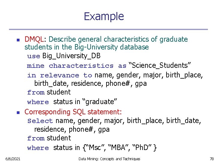
Example n n 6/6/2021 DMQL: Describe general characteristics of graduate students in the Big-University database use Big_University_DB mine characteristics as “Science_Students” in relevance to name, gender, major, birth_place, birth_date, residence, phone#, gpa from student where status in “graduate” Corresponding SQL statement: Select name, gender, major, birth_place, birth_date, residence, phone#, gpa from student where status in {“Msc”, “MBA”, “Ph. D” } Data Mining: Concepts and Techniques 78

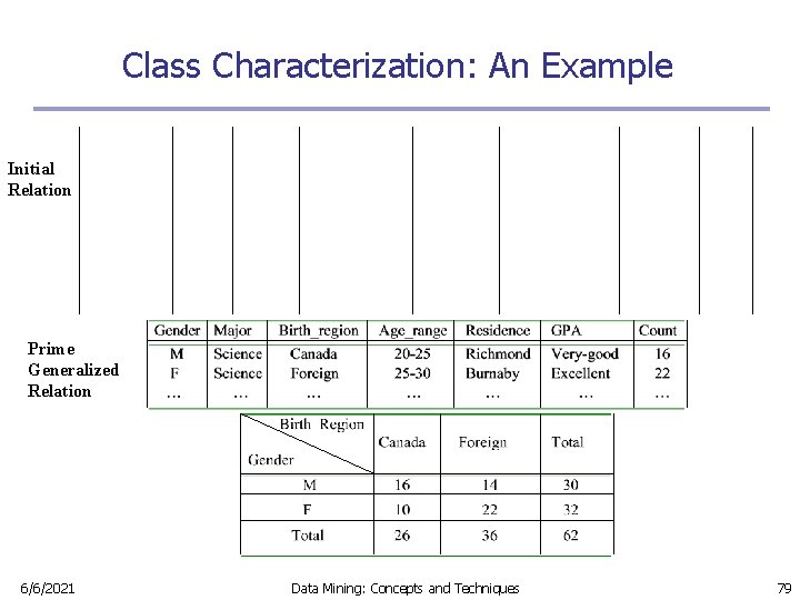
Class Characterization: An Example Initial Relation Prime Generalized Relation 6/6/2021 Data Mining: Concepts and Techniques 79

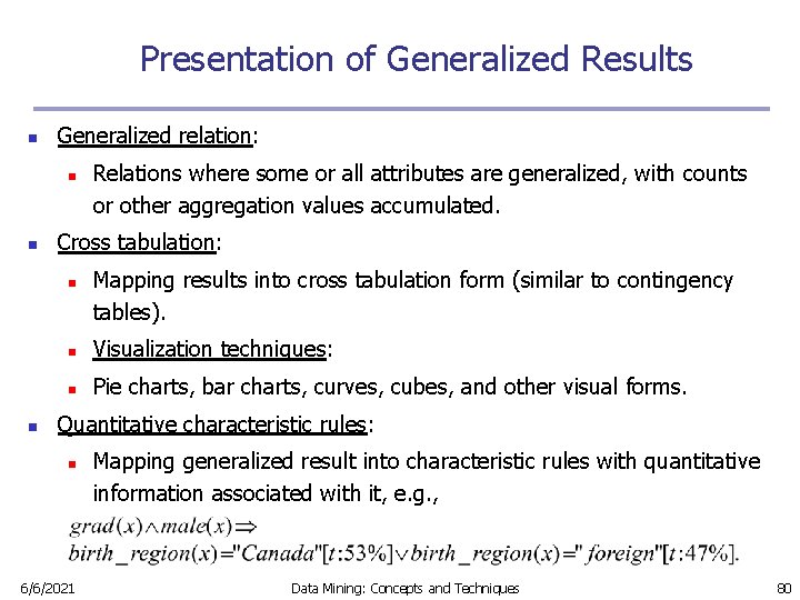
Presentation of Generalized Results n Generalized relation: n n Cross tabulation: n n Relations where some or all attributes are generalized, with counts or other aggregation values accumulated. Mapping results into cross tabulation form (similar to contingency tables). n Visualization techniques: n Pie charts, bar charts, curves, cubes, and other visual forms. Quantitative characteristic rules: n 6/6/2021 Mapping generalized result into characteristic rules with quantitative information associated with it, e. g. , Data Mining: Concepts and Techniques 80

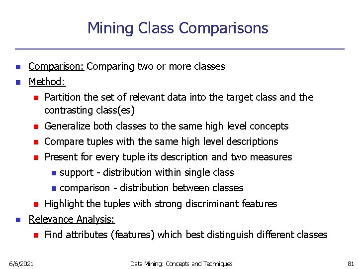
Mining Class Comparisons n Comparison: Comparing two or more classes n Method: n Partition the set of relevant data into the target class and the contrasting class(es) n Generalize both classes to the same high level concepts n Compare tuples with the same high level descriptions n Present for every tuple its description and two measures n n n support - distribution within single class n comparison - distribution between classes Highlight the tuples with strong discriminant features Relevance Analysis: n 6/6/2021 Find attributes (features) which best distinguish different classes Data Mining: Concepts and Techniques 81

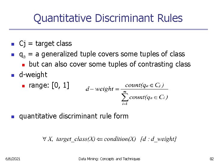
Quantitative Discriminant Rules n n Cj = target class qa = a generalized tuple covers some tuples of class n but can also cover some tuples of contrasting class d-weight n range: [0, 1] quantitative discriminant rule form 6/6/2021 Data Mining: Concepts and Techniques 82

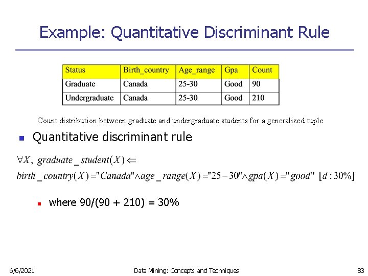
Example: Quantitative Discriminant Rule Count distribution between graduate and undergraduate students for a generalized tuple n Quantitative discriminant rule n 6/6/2021 where 90/(90 + 210) = 30% Data Mining: Concepts and Techniques 83

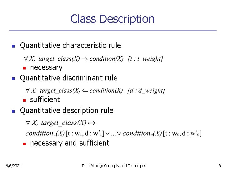
Class Description n Quantitative characteristic rule n necessary Quantitative discriminant rule n sufficient Quantitative description rule n n n 6/6/2021 necessary and sufficient Data Mining: Concepts and Techniques 84

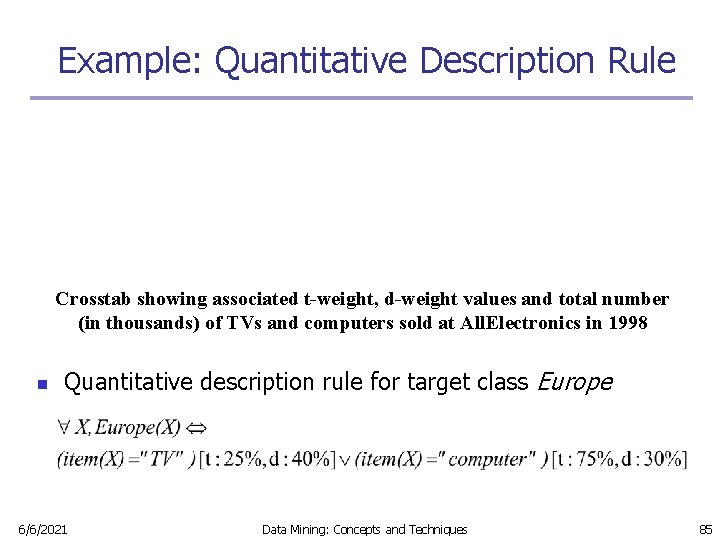
Example: Quantitative Description Rule Crosstab showing associated t-weight, d-weight values and total number (in thousands) of TVs and computers sold at All. Electronics in 1998 n Quantitative description rule for target class Europe 6/6/2021 Data Mining: Concepts and Techniques 85

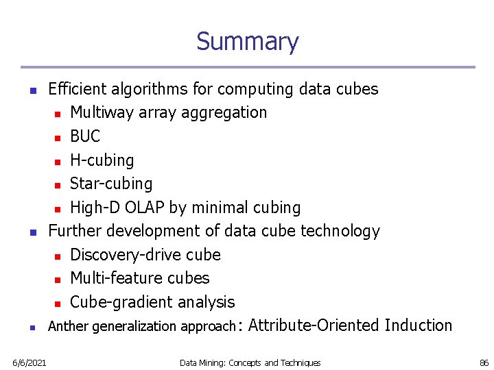
Summary n n n 6/6/2021 Efficient algorithms for computing data cubes n Multiway array aggregation n BUC n H-cubing n Star-cubing n High-D OLAP by minimal cubing Further development of data cube technology n Discovery-drive cube n Multi-feature cubes n Cube-gradient analysis Anther generalization approach: Attribute-Oriented Induction Data Mining: Concepts and Techniques 86

References (I) n S. Agarwal, R. Agrawal, P. M. Deshpande, A. Gupta, J. F. Naughton, R. Ramakrishnan, and S. Sarawagi. On the computation of multidimensional aggregates. VLDB’ 96 n D. Agrawal, A. E. Abbadi, A. Singh, and T. Yurek. Efficient view maintenance in data warehouses. SIGMOD’ 97 n R. Agrawal, A. Gupta, and S. Sarawagi. Modeling multidimensional databases. ICDE’ 97 n K. Beyer and R. Ramakrishnan. Bottom-Up Computation of Sparse and Iceberg CUBEs. . SIGMOD’ 99 n Y. Chen, G. Dong, J. Han, B. W. Wah, and J. Wang, Multi-Dimensional Regression Analysis of Time-Series Data Streams, VLDB'02 n G. Dong, J. Han, J. Lam, J. Pei, K. Wang. Mining Multi-dimensional Constrained Gradients in Data Cubes. VLDB’ 01 n J. Han, Y. Cai and N. Cercone, Knowledge Discovery in Databases: An Attribute-Oriented Approach, VLDB'92 n J. Han, J. Pei, G. Dong, K. Wang. Efficient Computation of Iceberg Cubes With Complex Measures. SIGMOD’ 01 6/6/2021 Data Mining: Concepts and Techniques 87

References (II) n n n n n L. V. S. Lakshmanan, J. Pei, and J. Han, Quotient Cube: How to Summarize the Semantics of a Data Cube, VLDB'02 X. Li, J. Han, and H. Gonzalez, High-Dimensional OLAP: A Minimal Cubing Approach, VLDB'04 K. Ross and D. Srivastava. Fast computation of sparse datacubes. VLDB’ 97 K. A. Ross, D. Srivastava, and D. Chatziantoniou. Complex aggregation at multiple granularities. EDBT'98 S. Sarawagi, R. Agrawal, and N. Megiddo. Discovery-driven exploration of OLAP data cubes. EDBT'98 G. Sathe and S. Sarawagi. Intelligent Rollups in Multidimensional OLAP Data. VLDB'01 D. Xin, J. Han, X. Li, B. W. Wah, Star-Cubing: Computing Iceberg Cubes by Top-Down and Bottom-Up Integration, VLDB'03 D. Xin, J. Han, Z. Shao, H. Liu, C-Cubing: Efficient Computation of Closed Cubes by Aggregation-Based Checking, ICDE'06 W. Wang, H. Lu, J. Feng, J. X. Yu, Condensed Cube: An Effective Approach to Reducing Data Cube Size. ICDE’ 02 Y. Zhao, P. M. Deshpande, and J. F. Naughton. An array-based algorithm for simultaneous multidimensional aggregates. SIGMOD’ 97 6/6/2021 Data Mining: Concepts and Techniques 88

6/6/2021 Data Mining: Concepts and Techniques 89