Data Mining Concepts and Techniques Chapter 3 Cont

Data Mining: Concepts and Techniques — Chapter 3 — Cont. More on Feature Selection: n n Chi-squared test Principal Component Analysis 1

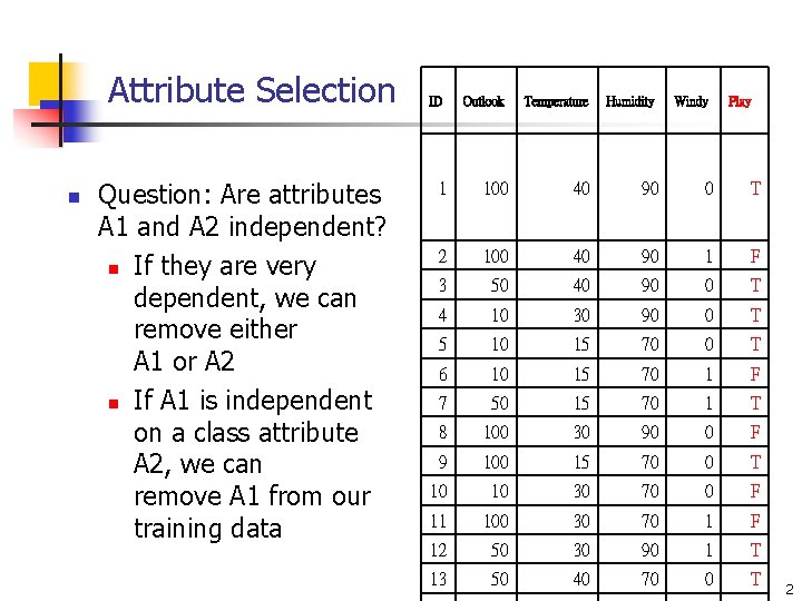
Attribute Selection n Question: Are attributes A 1 and A 2 independent? n If they are very dependent, we can remove either A 1 or A 2 n If A 1 is independent on a class attribute A 2, we can remove A 1 from our training data ID Outlook Temperature Humidity Windy Play 1 100 40 90 0 T 2 100 40 90 1 F 3 50 40 90 0 T 4 10 30 90 0 T 5 10 15 70 0 T 6 10 15 70 1 F 7 50 15 70 1 T 8 100 30 90 0 F 9 100 15 70 0 T 10 10 30 70 0 F 11 100 30 70 1 F 12 50 30 90 1 T 13 50 40 70 0 T 2

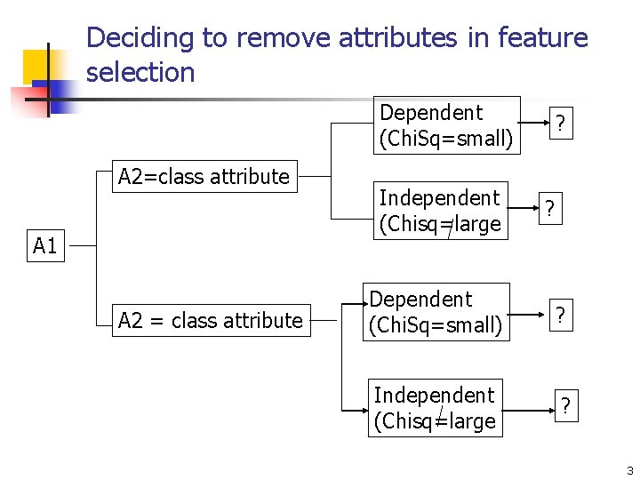
Deciding to remove attributes in feature selection Dependent (Chi. Sq=small) A 2=class attribute A 1 A 2 = class attribute Independent (Chisq=large ? ? Dependent (Chi. Sq=small) ? Independent (Chisq=large ? 3

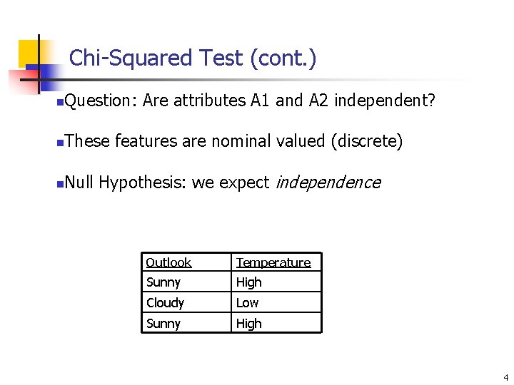
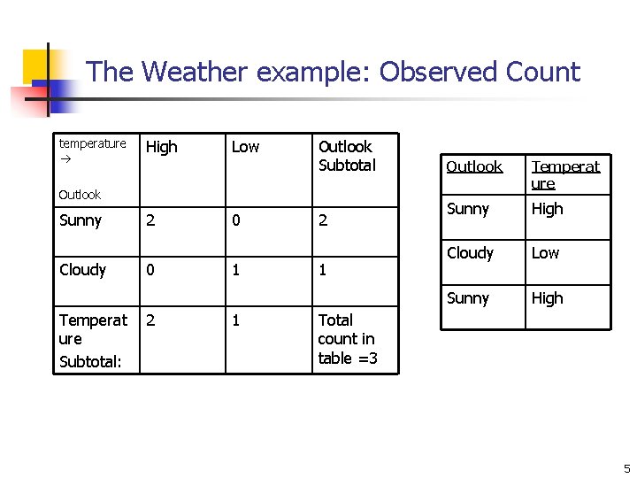
Chi-Squared Test (cont. ) n Question: Are attributes A 1 and A 2 independent? n These features are nominal valued (discrete) n Null Hypothesis: we expect independence Outlook Temperature Sunny High Cloudy Low Sunny High 4

The Weather example: Observed Count temperature High Low Outlook Subtotal Outlook Sunny Cloudy Temperat ure Subtotal: 2 0 1 1 2 1 Outlook Temperat ure Sunny High Cloudy Low Sunny High Total count in table =3 5

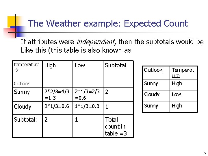
The Weather example: Expected Count If attributes were independent, then the subtotals would be Like this (this table is also known as temperature High Low Subtotal Outlook Temperat ure Sunny High Sunny 2*2/3=4/3 =1. 3 2*1/3=2/3 =0. 6 2 Cloudy Low Cloudy 2*1/3=0. 6 1*1/3=0. 3 1 Sunny High Subtotal: 2 1 Total count in table =3 6

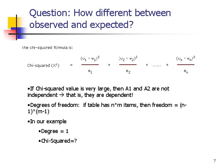
Question: How different between observed and expected? • If Chi-squared value is very large, then A 1 and A 2 are not independent that is, they are dependent! • Degrees of freedom: if table has n*m items, then freedom = (n 1)*(m-1) • In our example • Degree = 1 • Chi-Squared=? 7

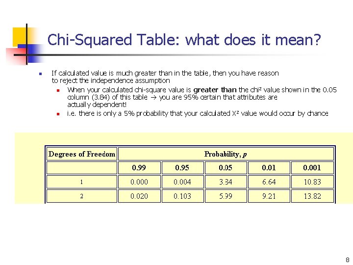
Chi-Squared Table: what does it mean? n If calculated value is much greater than in the table, then you have reason to reject the independence assumption n When your calculated chi-square value is greater than the chi 2 value shown in the 0. 05 column (3. 84) of this table you are 95% certain that attributes are actually dependent! n i. e. there is only a 5% probability that your calculated X 2 value would occur by chance 8

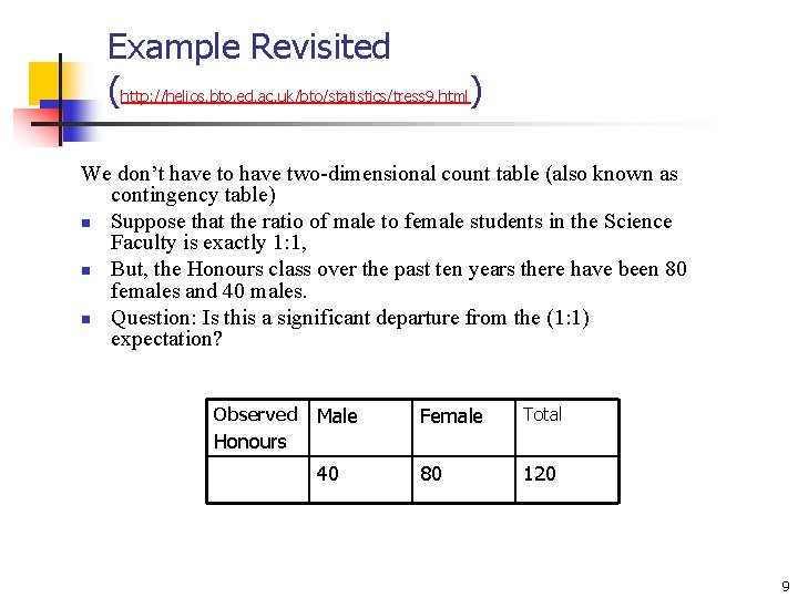
Example Revisited (http: //helios. bto. ed. ac. uk/bto/statistics/tress 9. html) We don’t have to have two-dimensional count table (also known as contingency table) n Suppose that the ratio of male to female students in the Science Faculty is exactly 1: 1, n But, the Honours class over the past ten years there have been 80 females and 40 males. n Question: Is this a significant departure from the (1: 1) expectation? Observed Male Female Total 40 80 120 Honours 9

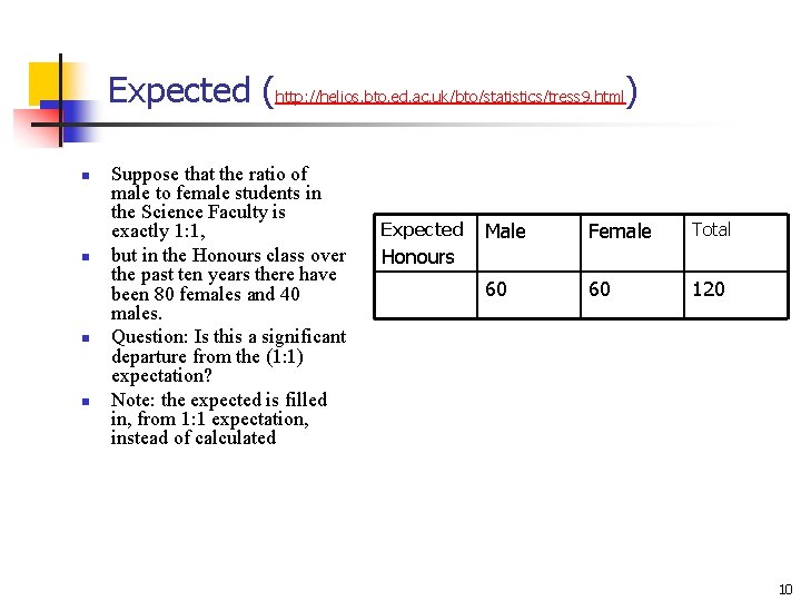
Expected (http: //helios. bto. ed. ac. uk/bto/statistics/tress 9. html) n n Suppose that the ratio of male to female students in the Science Faculty is exactly 1: 1, but in the Honours class over the past ten years there have been 80 females and 40 males. Question: Is this a significant departure from the (1: 1) expectation? Note: the expected is filled in, from 1: 1 expectation, instead of calculated Expected Male Female Total 60 60 120 Honours 10

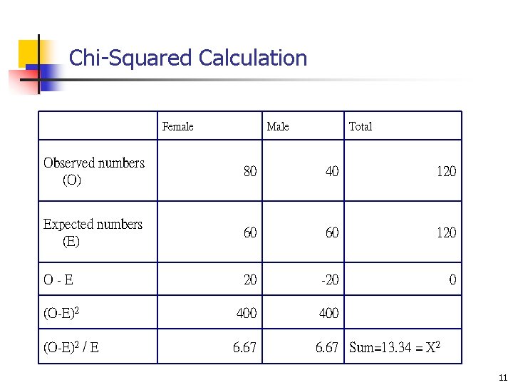
Chi-Squared Calculation 　 Female Male Total Observed numbers (O) 80 40 120 Expected numbers (E) 60 60 120 O-E 20 -20 0 (O-E)2 400 　 (O-E)2 / E 6. 67 Sum=13. 34 = X 2 11

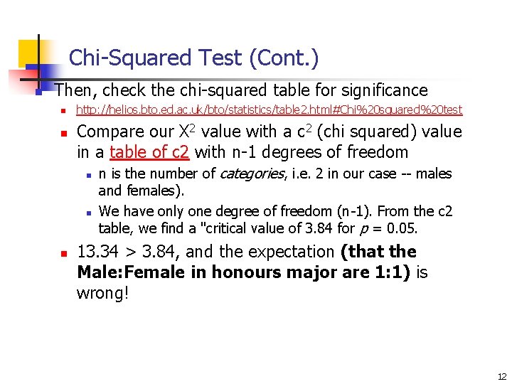
Chi-Squared Test (Cont. ) n Then, check the chi-squared table for significance n n http: //helios. bto. ed. ac. uk/bto/statistics/table 2. html#Chi%20 squared%20 test Compare our X 2 value with a c 2 (chi squared) value in a table of c 2 with n-1 degrees of freedom n n is the number of categories, i. e. 2 in our case -- males and females). We have only one degree of freedom (n-1). From the c 2 table, we find a "critical value of 3. 84 for p = 0. 05. 13. 34 > 3. 84, and the expectation (that the Male: Female in honours major are 1: 1) is wrong! 12

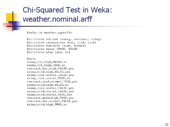
Chi-Squared Test in Weka: weather. nominal. arff 13

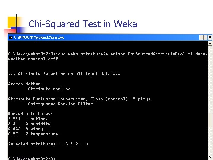
Chi-Squared Test in Weka 14

Chi-Squared Test in Weka 15

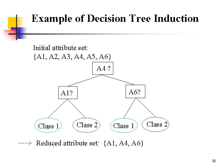
Example of Decision Tree Induction Initial attribute set: {A 1, A 2, A 3, A 4, A 5, A 6} A 4 ? A 6? A 1? Class 1 > Class 2 Class 1 Class 2 Reduced attribute set: {A 1, A 4, A 6} 16

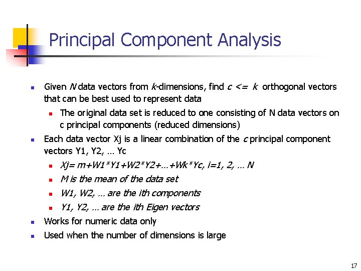
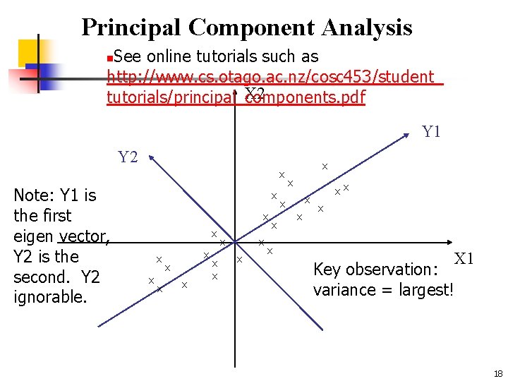
Principal Component Analysis n Given N data vectors from k-dimensions, find c <= k orthogonal vectors that can be best used to represent data n n The original data set is reduced to one consisting of N data vectors on c principal components (reduced dimensions) Each data vector Xj is a linear combination of the c principal component vectors Y 1, Y 2, … Yc n n Xj= m+W 1*Y 1+W 2*Y 2+…+Wk*Yc, i=1, 2, … N M is the mean of the data set W 1, W 2, … are the ith components Y 1, Y 2, … are the ith Eigen vectors n Works for numeric data only n Used when the number of dimensions is large 17

Principal Component Analysis See online tutorials such as http: //www. cs. otago. ac. nz/cosc 453/student_ X 2 tutorials/principal_components. pdf n Y 1 Y 2 x Note: Y 1 is the first eigen vector, Y 2 is the second. Y 2 ignorable. x x x x x xx x X 1 Key observation: variance = largest! 18

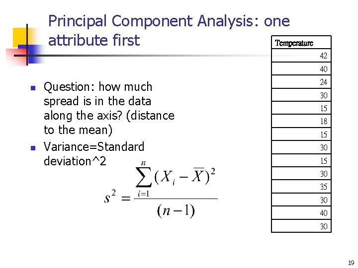
Principal Component Analysis: one Temperature attribute first 42 40 n n Question: how much spread is in the data along the axis? (distance to the mean) Variance=Standard deviation^2 24 30 15 18 15 30 35 30 40 30 19

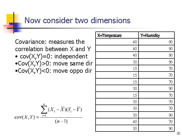
Now consider two dimensions X=Temperature Covariance: measures the correlation between X and Y • cov(X, Y)=0: independent • Cov(X, Y)>0: move same dir • Cov(X, Y)<0: move oppo dir Y=Humidity 40 90 30 90 15 70 30 90 15 70 30 90 40 70 30 90 20

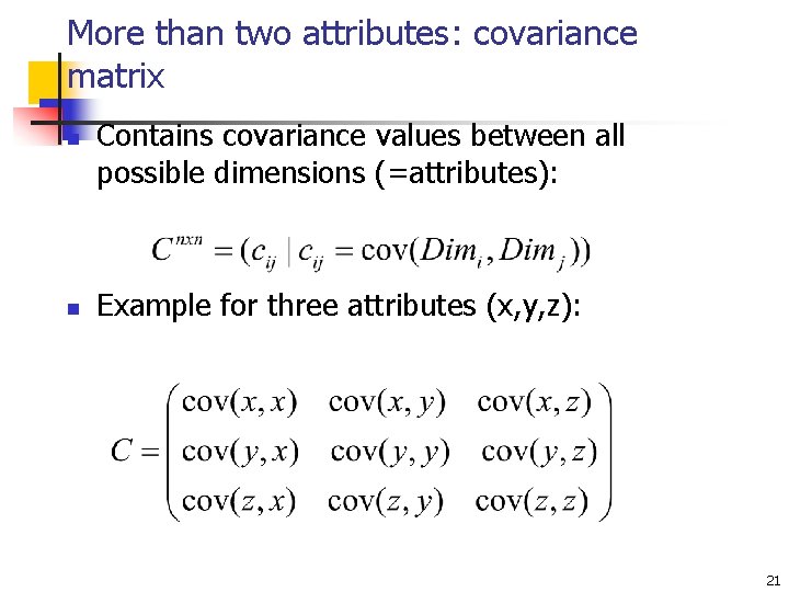
More than two attributes: covariance matrix n n Contains covariance values between all possible dimensions (=attributes): Example for three attributes (x, y, z): 21

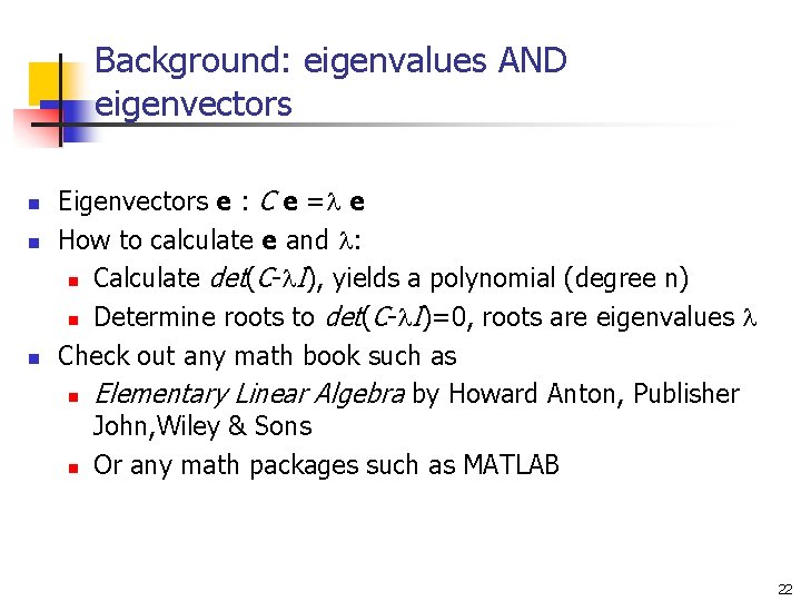
Background: eigenvalues AND eigenvectors n n n Eigenvectors e : C e = e How to calculate e and : n Calculate det(C- I), yields a polynomial (degree n) n Determine roots to det(C- I)=0, roots are eigenvalues Check out any math book such as n Elementary Linear Algebra by Howard Anton, Publisher John, Wiley & Sons n Or any math packages such as MATLAB 22

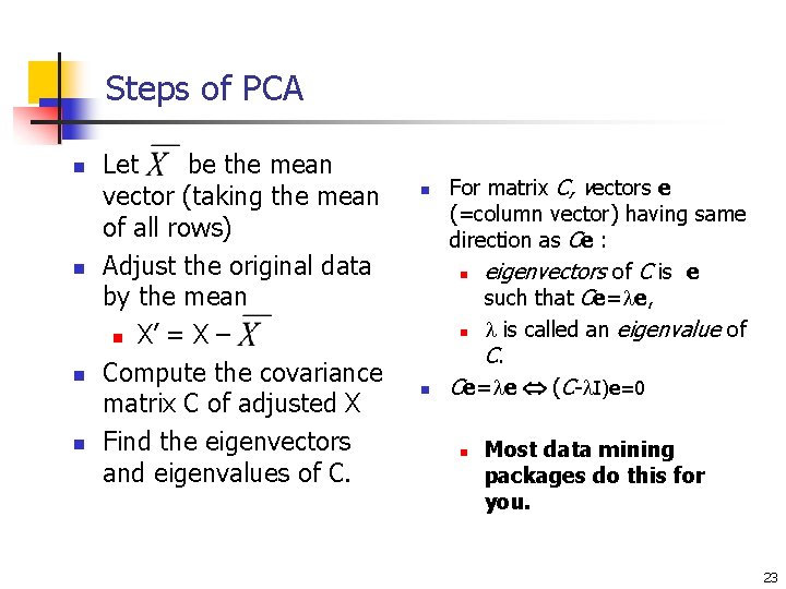
Steps of PCA n n Let be the mean vector (taking the mean of all rows) Adjust the original data by the mean n X’ = X – Compute the covariance matrix C of adjusted X Find the eigenvectors and eigenvalues of C. n n For matrix C, vectors e (=column vector) having same direction as Ce : n eigenvectors of C is e such that Ce= e, n is called an eigenvalue of C. Ce= e (C- I)e=0 n Most data mining packages do this for you. 23

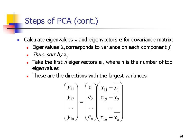
Steps of PCA (cont. ) n Calculate eigenvalues and eigenvectors e for covariance matrix: n Eigenvalues j corresponds to variance on each component j n Thus, sort by j n Take the first n eigenvectors ei; where n is the number of top eigenvalues n These are the directions with the largest variances 24

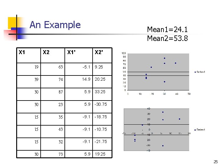
An Example X 1 X 2 Mean 1=24. 1 Mean 2=53. 8 X 1' X 2' 19 63 -5. 1 9. 25 39 74 14. 9 20. 25 30 87 5. 9 33. 25 30 23 5. 9 -30. 75 15 35 -9. 1 -18. 75 15 43 -9. 1 -10. 75 15 32 -9. 1 -21. 75 30 73 5. 9 19. 25 25

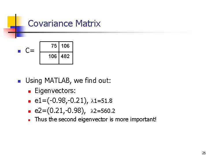
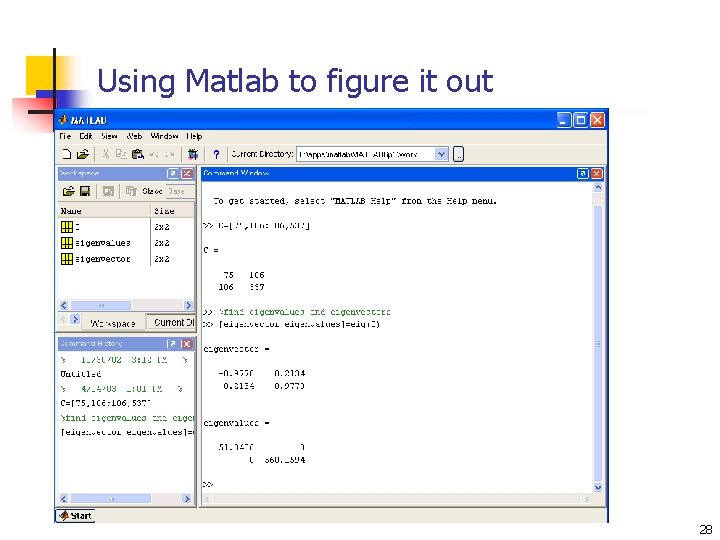
Covariance Matrix n n C= 75 106 482 Using MATLAB, we find out: n Eigenvectors: n e 1=(-0. 98, -0. 21), 1=51. 8 n e 2=(0. 21, -0. 98), 2=560. 2 n Thus the second eigenvector is more important! 26

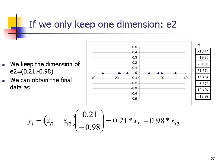
If we only keep one dimension: e 2 yi -10. 14 -16. 72 n n We keep the dimension of e 2=(0. 21, -0. 98) We can obtain the final data as -31. 35 31. 374 16. 464 8. 624 19. 404 -17. 63 27

Using Matlab to figure it out 28

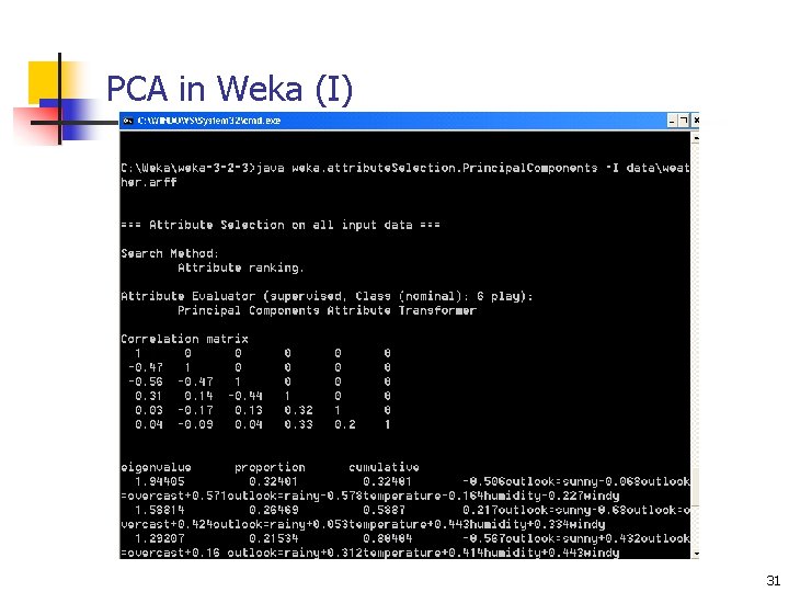
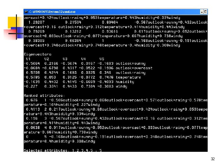
PCA in Weka 29

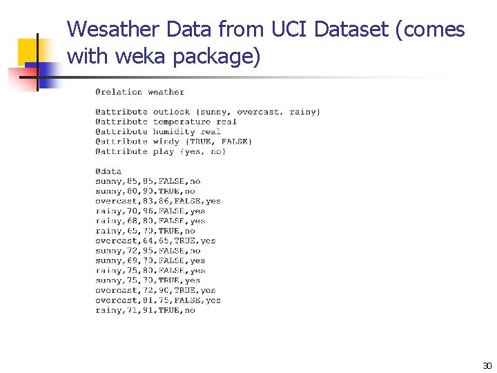
Wesather Data from UCI Dataset (comes with weka package) 30

PCA in Weka (I) 31

32

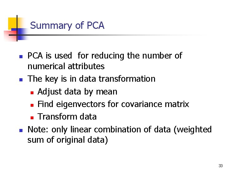
Summary of PCA n n n PCA is used for reducing the number of numerical attributes The key is in data transformation n Adjust data by mean n Find eigenvectors for covariance matrix n Transform data Note: only linear combination of data (weighted sum of original data) 33

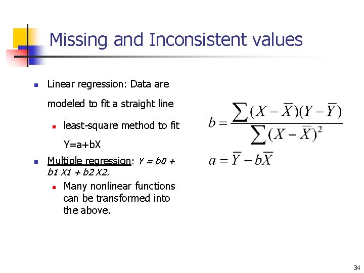
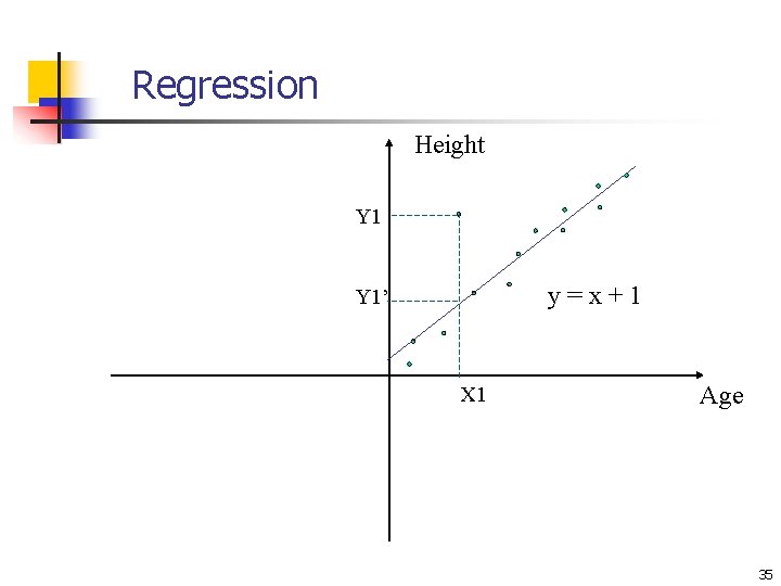
Missing and Inconsistent values n Linear regression: Data are modeled to fit a straight line n least-square method to fit Y=a+b. X n Multiple regression: Y = b 0 + b 1 X 1 + b 2 X 2. n Many nonlinear functions can be transformed into the above. 34

Regression Height Y 1 y=x+1 Y 1’ X 1 Age 35

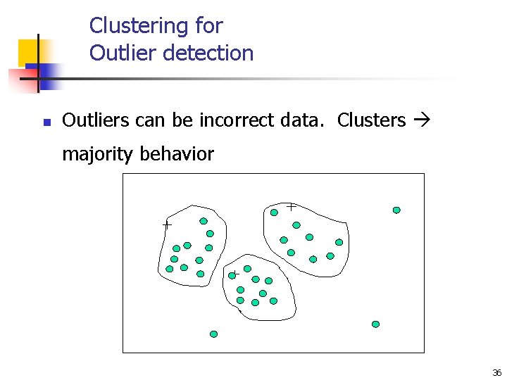
Clustering for Outlier detection n Outliers can be incorrect data. Clusters majority behavior 36

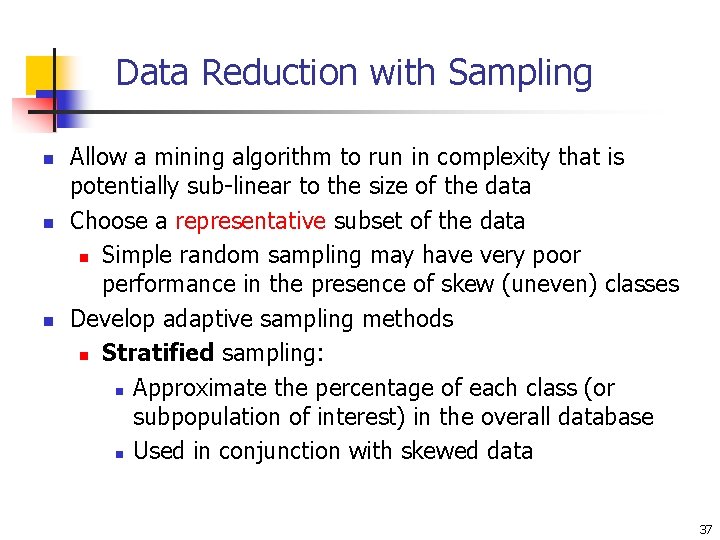
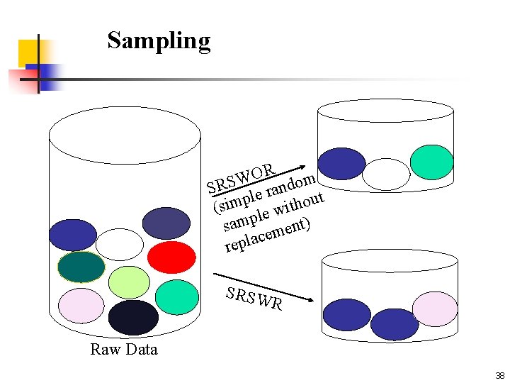
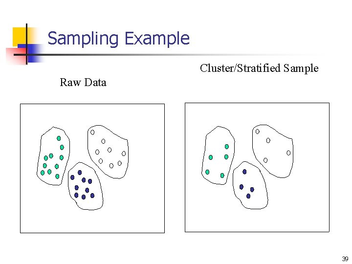
Data Reduction with Sampling n n n Allow a mining algorithm to run in complexity that is potentially sub-linear to the size of the data Choose a representative subset of the data n Simple random sampling may have very poor performance in the presence of skew (uneven) classes Develop adaptive sampling methods n Stratified sampling: n Approximate the percentage of each class (or subpopulation of interest) in the overall database n Used in conjunction with skewed data 37

Sampling R O W SRS le random t p u o m i h t s ( wi e l p sam ment) e c a l p re SRSW R Raw Data 38

Sampling Example Cluster/Stratified Sample Raw Data 39

Summary n Data preparation is a big issue for data mining n Data preparation includes n Data warehousing n Data reduction and feature selection n Discretization n Missing values n Incorrect values n Sampling 40