Data Mining Concepts and Techniques Chapter 2 Jiawei

Data Mining: Concepts and Techniques — Chapter 2 — Jiawei Han, Micheline Kamber, and Jian Pei University of Illinois at Urbana-Champaign Simon Fraser University © 2011 Han, Kamber, and Pei. All rights reserved. 1

Chapter 2: Getting to Know Your Data n Data Objects and Attribute Types n Basic Statistical Descriptions of Data n Data Visualization n Measuring Data Similarity and Dissimilarity n Summary 2

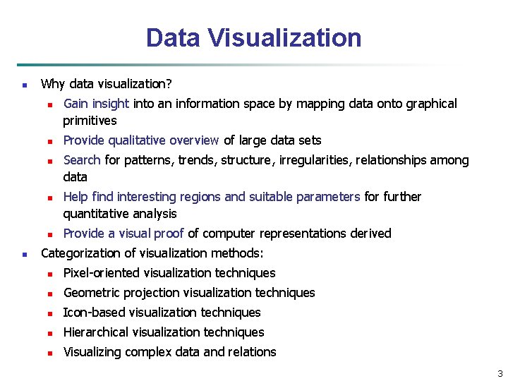
Data Visualization n Why data visualization? n n n Gain insight into an information space by mapping data onto graphical primitives Provide qualitative overview of large data sets Search for patterns, trends, structure, irregularities, relationships among data Help find interesting regions and suitable parameters for further quantitative analysis Provide a visual proof of computer representations derived Categorization of visualization methods: n Pixel-oriented visualization techniques n Geometric projection visualization techniques n Icon-based visualization techniques n Hierarchical visualization techniques n Visualizing complex data and relations 3

Chapter 2: Getting to Know Your Data n Data Objects and Attribute Types n Basic Statistical Descriptions of Data n Data Visualization n Measuring Data Similarity and Dissimilarity n Summary 4

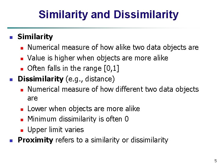
Similarity and Dissimilarity n n n Similarity n Numerical measure of how alike two data objects are n Value is higher when objects are more alike n Often falls in the range [0, 1] Dissimilarity (e. g. , distance) n Numerical measure of how different two data objects are n Lower when objects are more alike n Minimum dissimilarity is often 0 n Upper limit varies Proximity refers to a similarity or dissimilarity 5

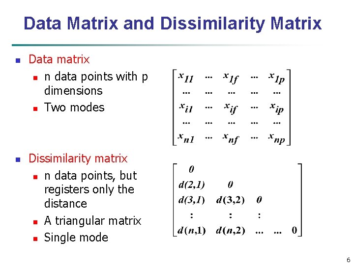
Data Matrix and Dissimilarity Matrix n n Data matrix n n data points with p dimensions n Two modes Dissimilarity matrix n n data points, but registers only the distance n A triangular matrix n Single mode 6

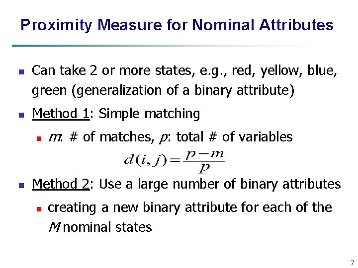
Proximity Measure for Nominal Attributes n n Can take 2 or more states, e. g. , red, yellow, blue, green (generalization of a binary attribute) Method 1: Simple matching n n m: # of matches, p: total # of variables Method 2: Use a large number of binary attributes n creating a new binary attribute for each of the M nominal states 7

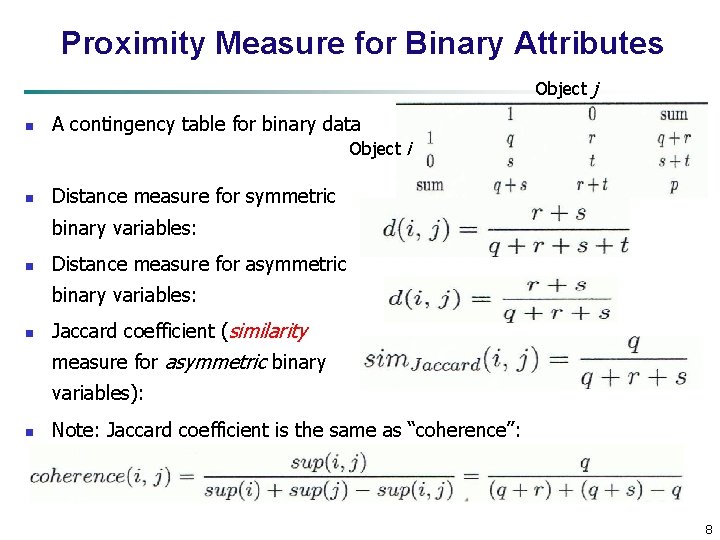
Proximity Measure for Binary Attributes Object j n A contingency table for binary data Object i n Distance measure for symmetric binary variables: n Distance measure for asymmetric binary variables: n Jaccard coefficient (similarity measure for asymmetric binary variables): n Note: Jaccard coefficient is the same as “coherence”: 8

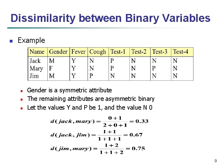
Dissimilarity between Binary Variables n Example n n n Gender is a symmetric attribute The remaining attributes are asymmetric binary Let the values Y and P be 1, and the value N 0 9

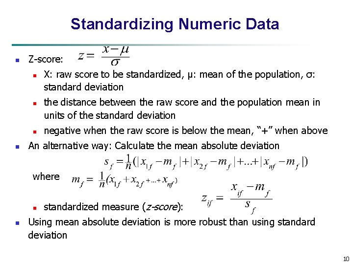
Standardizing Numeric Data n Z-score: n n X: raw score to be standardized, μ: mean of the population, σ: standard deviation the distance between the raw score and the population mean in units of the standard deviation negative when the raw score is below the mean, “+” when above An alternative way: Calculate the mean absolute deviation where n n standardized measure (z-score): Using mean absolute deviation is more robust than using standard deviation 10

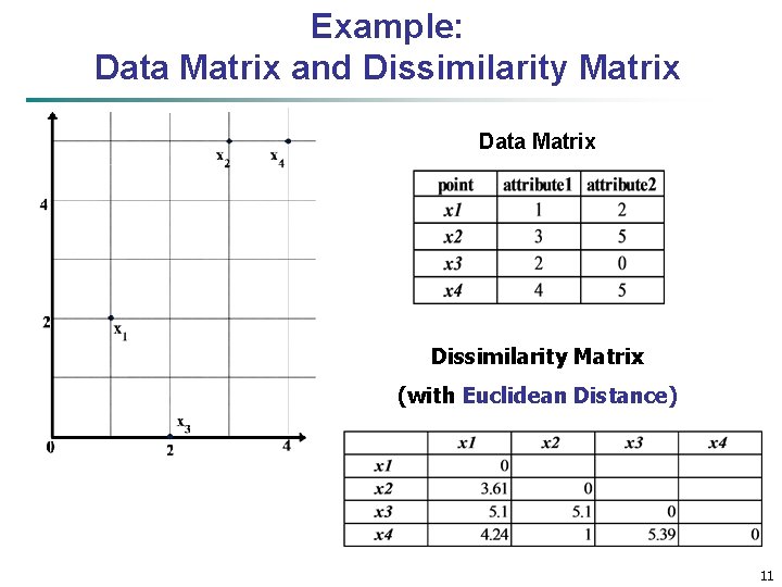
Example: Data Matrix and Dissimilarity Matrix Data Matrix Dissimilarity Matrix (with Euclidean Distance) 11

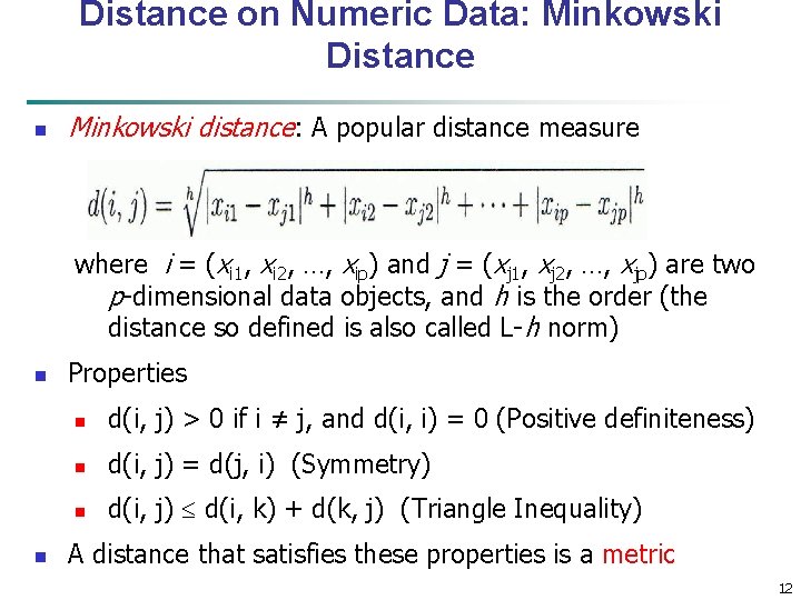
Distance on Numeric Data: Minkowski Distance n Minkowski distance: A popular distance measure where i = (xi 1, xi 2, …, xip) and j = (xj 1, xj 2, …, xjp) are two p-dimensional data objects, and h is the order (the distance so defined is also called L-h norm) n n Properties n d(i, j) > 0 if i ≠ j, and d(i, i) = 0 (Positive definiteness) n d(i, j) = d(j, i) (Symmetry) n d(i, j) d(i, k) + d(k, j) (Triangle Inequality) A distance that satisfies these properties is a metric 12

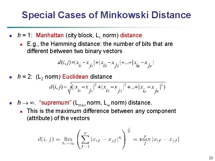
Special Cases of Minkowski Distance n n n h = 1: Manhattan (city block, L 1 norm) distance n E. g. , the Hamming distance: the number of bits that are different between two binary vectors h = 2: (L 2 norm) Euclidean distance h . “supremum” (Lmax norm, L norm) distance. n This is the maximum difference between any component (attribute) of the vectors 13

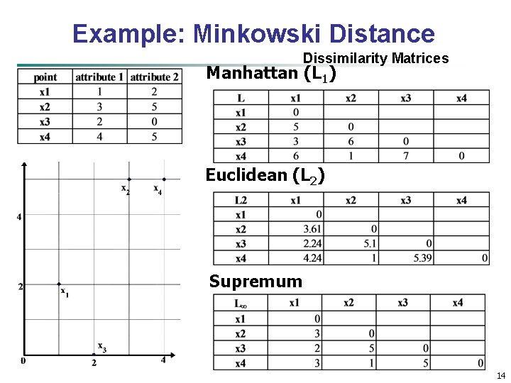
Example: Minkowski Distance Dissimilarity Matrices Manhattan (L 1) Euclidean (L 2) Supremum 14

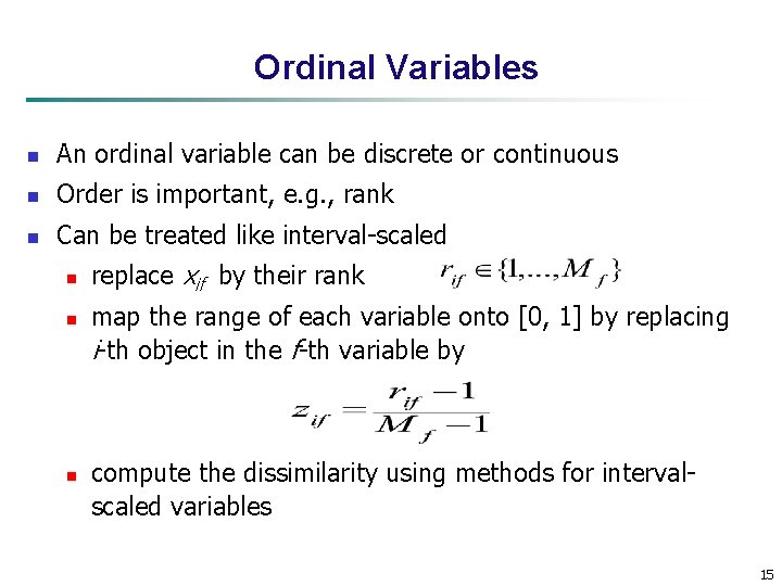
Ordinal Variables n An ordinal variable can be discrete or continuous n Order is important, e. g. , rank n Can be treated like interval-scaled n n n replace xif by their rank map the range of each variable onto [0, 1] by replacing i-th object in the f-th variable by compute the dissimilarity using methods for intervalscaled variables 15

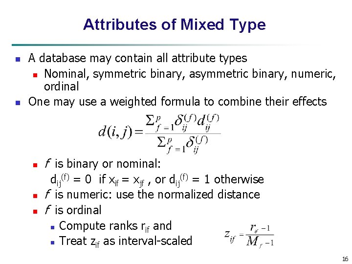
Attributes of Mixed Type n n A database may contain all attribute types n Nominal, symmetric binary, asymmetric binary, numeric, ordinal One may use a weighted formula to combine their effects n n n f is binary or nominal: dij(f) = 0 if xif = xjf , or dij(f) = 1 otherwise f is numeric: use the normalized distance f is ordinal n Compute ranks rif and n Treat zif as interval-scaled 16

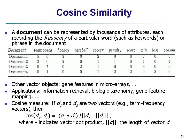
Cosine Similarity n n A document can be represented by thousands of attributes, each recording the frequency of a particular word (such as keywords) or phrase in the document. Other vector objects: gene features in micro-arrays, … Applications: information retrieval, biologic taxonomy, gene feature mapping, . . . Cosine measure: If d 1 and d 2 are two vectors (e. g. , term-frequency vectors), then cos(d 1, d 2) = (d 1 d 2) /||d 1|| ||d 2|| , where indicates vector dot product, ||d||: the length of vector d 17

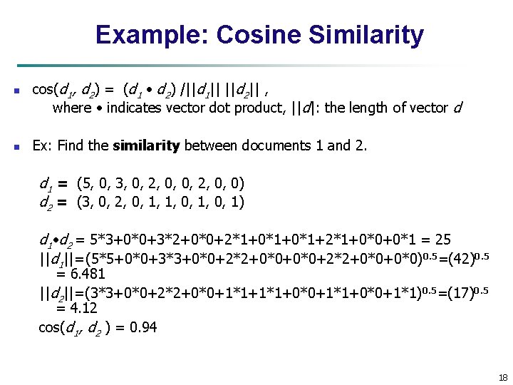
Example: Cosine Similarity n n cos(d 1, d 2) = (d 1 d 2) /||d 1|| ||d 2|| , where indicates vector dot product, ||d|: the length of vector d Ex: Find the similarity between documents 1 and 2. d 1 = (5, 0, 3, 0, 2, 0, 0) d 2 = (3, 0, 2, 0, 1, 1, 0, 1) d 1 d 2 = 5*3+0*0+3*2+0*0+2*1+0*1+2*1+0*0+0*1 = 25 ||d 1||= (5*5+0*0+3*3+0*0+2*2+0*0+0*0) 0. 5=(42)0. 5 = 6. 481 ||d 2||=(3*3+0*0+2*2+0*0+1*1+0*0+1*1) 0. 5=(17)0. 5 = 4. 12 cos(d 1, d 2 ) = 0. 94 18

Chapter 2: Getting to Know Your Data n Data Objects and Attribute Types n Basic Statistical Descriptions of Data n Data Visualization n Measuring Data Similarity and Dissimilarity n Summary 19

Summary n Data attribute types: nominal, binary, ordinal, interval-scaled, ratioscaled n Many types of data sets, e. g. , numerical, text, graph, Web, image. n Gain insight into the data by: n Basic statistical data description: central tendency, dispersion, graphical displays n Data visualization: map data onto graphical primitives n Measure data similarity n Above steps are the beginning of data preprocessing. n Many methods have been developed but still an active area of research. 20

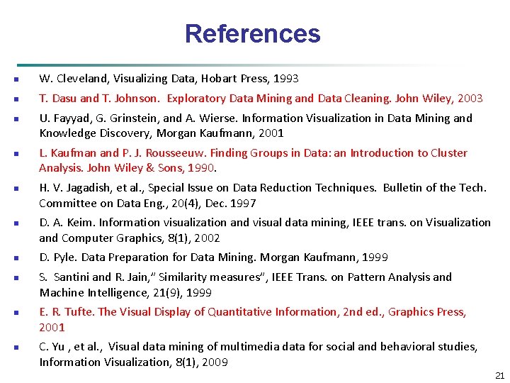
References n W. Cleveland, Visualizing Data, Hobart Press, 1993 n T. Dasu and T. Johnson. Exploratory Data Mining and Data Cleaning. John Wiley, 2003 n n n n U. Fayyad, G. Grinstein, and A. Wierse. Information Visualization in Data Mining and Knowledge Discovery, Morgan Kaufmann, 2001 L. Kaufman and P. J. Rousseeuw. Finding Groups in Data: an Introduction to Cluster Analysis. John Wiley & Sons, 1990. H. V. Jagadish, et al. , Special Issue on Data Reduction Techniques. Bulletin of the Tech. Committee on Data Eng. , 20(4), Dec. 1997 D. A. Keim. Information visualization and visual data mining, IEEE trans. on Visualization and Computer Graphics, 8(1), 2002 D. Pyle. Data Preparation for Data Mining. Morgan Kaufmann, 1999 S. Santini and R. Jain, ” Similarity measures”, IEEE Trans. on Pattern Analysis and Machine Intelligence, 21(9), 1999 E. R. Tufte. The Visual Display of Quantitative Information, 2 nd ed. , Graphics Press, 2001 C. Yu , et al. , Visual data mining of multimedia data for social and behavioral studies, Information Visualization, 8(1), 2009 21