Data Mining Concepts and Techniques Chapter 2 Jiawei

Data Mining: Concepts and Techniques — Chapter 2 — Jiawei Han, Micheline Kamber, and Jian Pei University of Illinois at Urbana-Champaign Simon Fraser University © 2013 Han, Kamber, and Pei. All rights reserved. 1

Chapter 2: Getting to Know Your Data n Data Objects and Attribute Types n Basic Statistical Descriptions of Data n Data Visualization n Measuring Data Similarity and Dissimilarity n Summary 2

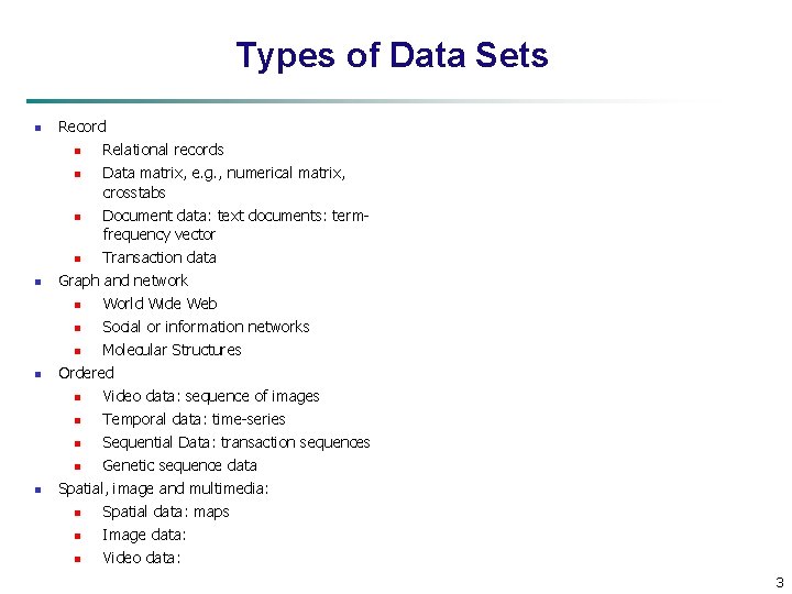
Types of Data Sets n n Record n Relational records n Data matrix, e. g. , numerical matrix, crosstabs n Document data: text documents: termfrequency vector n Transaction data Graph and network n World Wide Web n Social or information networks n Molecular Structures Ordered n Video data: sequence of images n Temporal data: time-series n Sequential Data: transaction sequences n Genetic sequence data Spatial, image and multimedia: n Spatial data: maps n Image data: n Video data: 3

Data Objects n Data sets are made up of data objects. n A data object represents an entity. n Examples: n n sales database: customers, store items, sales n medical database: patients, treatments n university database: students, professors, courses Also called samples , examples, instances, data points, objects, tuples. n Data objects are described by attributes. n Database rows -> data objects; columns ->attributes. 4

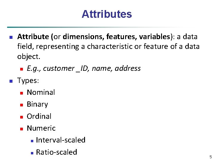
Attributes n n Attribute (or dimensions, features, variables): a data field, representing a characteristic or feature of a data object. n E. g. , customer _ID, name, address Types: n Nominal n Binary n Ordinal n Numeric n Interval-scaled n Ratio-scaled 5

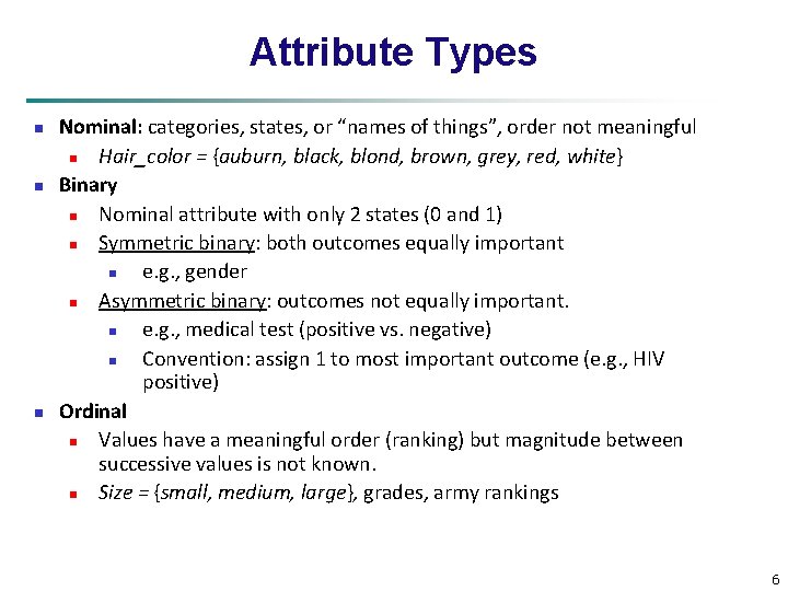
Attribute Types n n n Nominal: categories, states, or “names of things”, order not meaningful n Hair_color = {auburn, black, blond, brown, grey, red, white} Binary n Nominal attribute with only 2 states (0 and 1) n Symmetric binary: both outcomes equally important n e. g. , gender n Asymmetric binary: outcomes not equally important. n e. g. , medical test (positive vs. negative) n Convention: assign 1 to most important outcome (e. g. , HIV positive) Ordinal n Values have a meaningful order (ranking) but magnitude between successive values is not known. n Size = {small, medium, large}, grades, army rankings 6

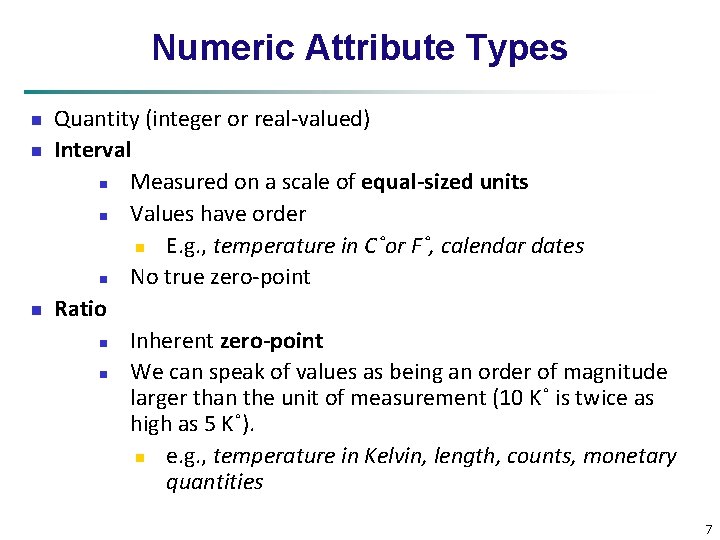
Numeric Attribute Types n n n Quantity (integer or real-valued) Interval n Measured on a scale of equal-sized units n Values have order n E. g. , temperature in C˚or F˚, calendar dates n No true zero-point Ratio n Inherent zero-point n We can speak of values as being an order of magnitude larger than the unit of measurement (10 K˚ is twice as high as 5 K˚). n e. g. , temperature in Kelvin, length, counts, monetary quantities 7

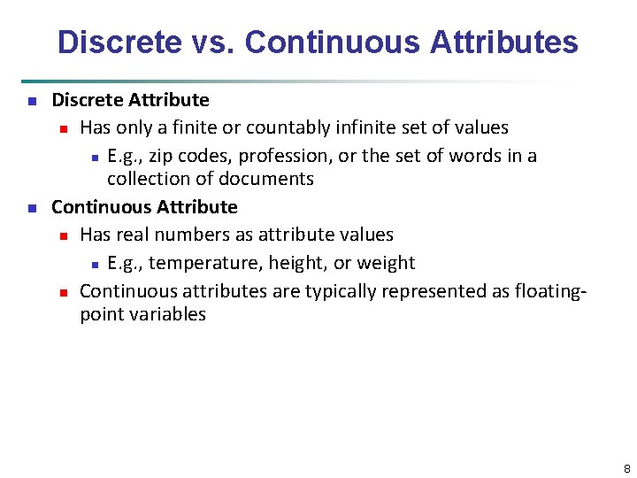
Discrete vs. Continuous Attributes n n Discrete Attribute n Has only a finite or countably infinite set of values n E. g. , zip codes, profession, or the set of words in a collection of documents Continuous Attribute n Has real numbers as attribute values n E. g. , temperature, height, or weight n Continuous attributes are typically represented as floatingpoint variables 8

Chapter 2: Getting to Know Your Data n Data Objects and Attribute Types n Basic Statistical Descriptions of Data n Data Visualization n Measuring Data Similarity and Dissimilarity n Summary 9

Basic Statistical Descriptions of Data Measures of central tendency n Mean, median, mode n Dispersion of data n range, quartiles and interquartile range, five-number summary and boxplots, variance and standard deviation n 10

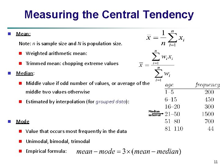
Measuring the Central Tendency n Mean: Note: n is sample size and N is population size. n n Weighted arithmetic mean: n Trimmed mean: chopping extreme values Median: n Middle value if odd number of values, or average of the middle two values otherwise n Estimated by interpolation (for grouped data): Median interval n Mode n Value that occurs most frequently in the data n Unimodal, bimodal, trimodal n Empirical formula: 11

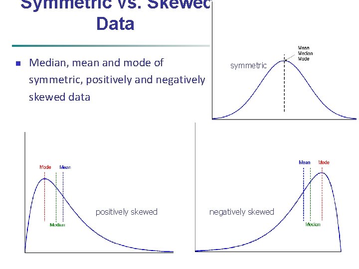
Symmetric vs. Skewed Data n Median, mean and mode of symmetric, positively and negatively skewed data positively skewed 04 December 2020 symmetric negatively skewed Data Mining: Concepts and Techniques 12

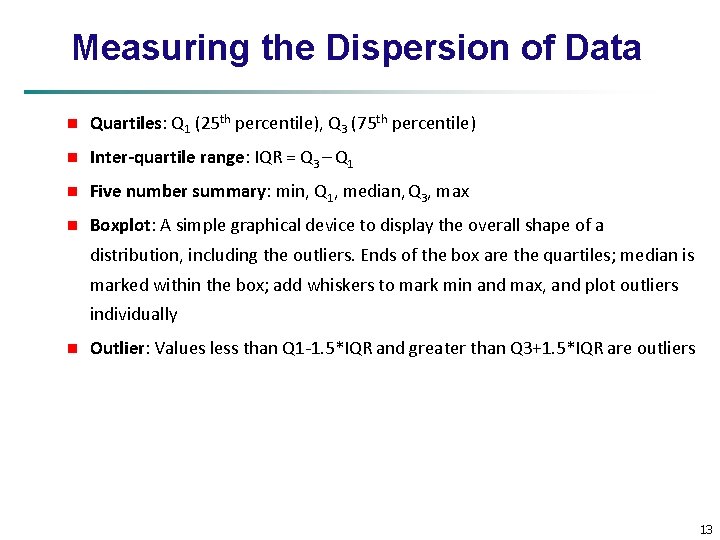
Measuring the Dispersion of Data n Quartiles: Q 1 (25 th percentile), Q 3 (75 th percentile) n Inter-quartile range: IQR = Q 3 – Q 1 n Five number summary: min, Q 1, median, Q 3, max n Boxplot: A simple graphical device to display the overall shape of a distribution, including the outliers. Ends of the box are the quartiles; median is marked within the box; add whiskers to mark min and max, and plot outliers individually n Outlier: Values less than Q 1 -1. 5*IQR and greater than Q 3+1. 5*IQR are outliers 13

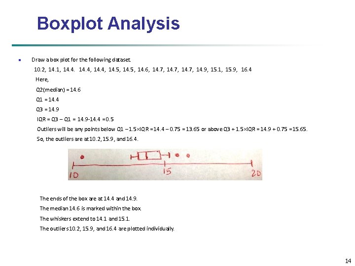
Boxplot Analysis n Draw a box plot for the following dataset. 10. 2, 14. 1, 14. 4, 14. 5, 14. 6, 14. 7, 14. 9, 15. 1, 15. 9, 16. 4 Here, Q 2(median) = 14. 6 Q 1 = 14. 4 Q 3 = 14. 9 IQR = Q 3 – Q 1 = 14. 9 -14. 4 = 0. 5 Outliers will be any points below Q 1 – 1. 5×IQR = 14. 4 – 0. 75 = 13. 65 or above Q 3 + 1. 5×IQR = 14. 9 + 0. 75 = 15. 65. So, the outliers are at 10. 2, 15. 9, and 16. 4. The ends of the box are at 14. 4 and 14. 9. The median 14. 6 is marked within the box. The whiskers extend to 14. 1 and 15. 1. The outliers 10. 2, 15. 9, and 16. 4 are plotted individually. 14

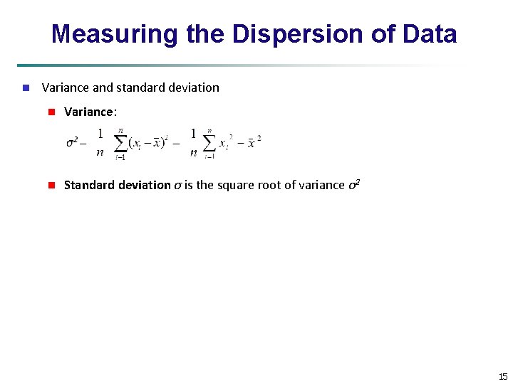
Measuring the Dispersion of Data n Variance and standard deviation n Variance: n Standard deviation σ is the square root of variance σ2 15

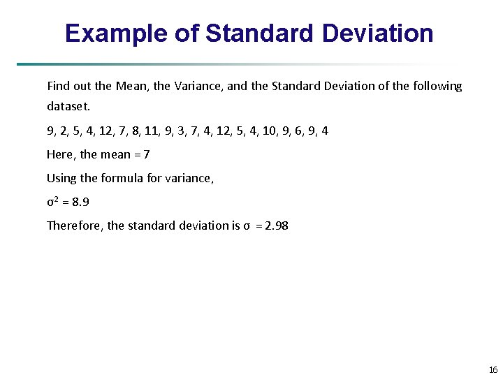
Example of Standard Deviation Find out the Mean, the Variance, and the Standard Deviation of the following dataset. 9, 2, 5, 4, 12, 7, 8, 11, 9, 3, 7, 4, 12, 5, 4, 10, 9, 6, 9, 4 Here, the mean = 7 Using the formula for variance, σ2 = 8. 9 Therefore, the standard deviation is σ = 2. 98 16

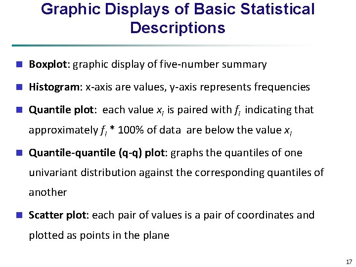
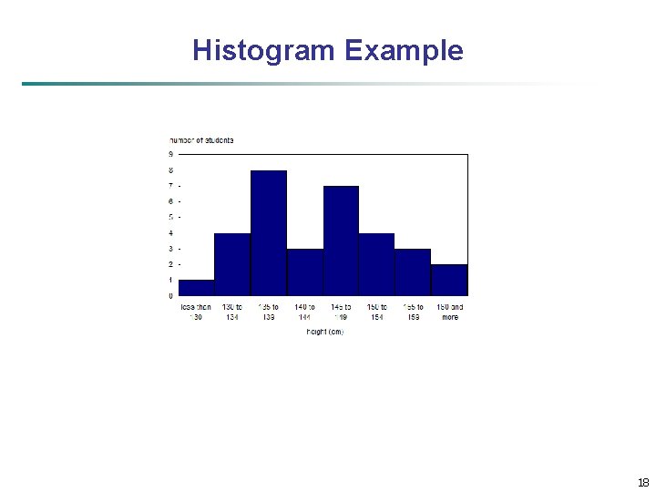
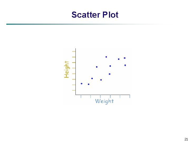
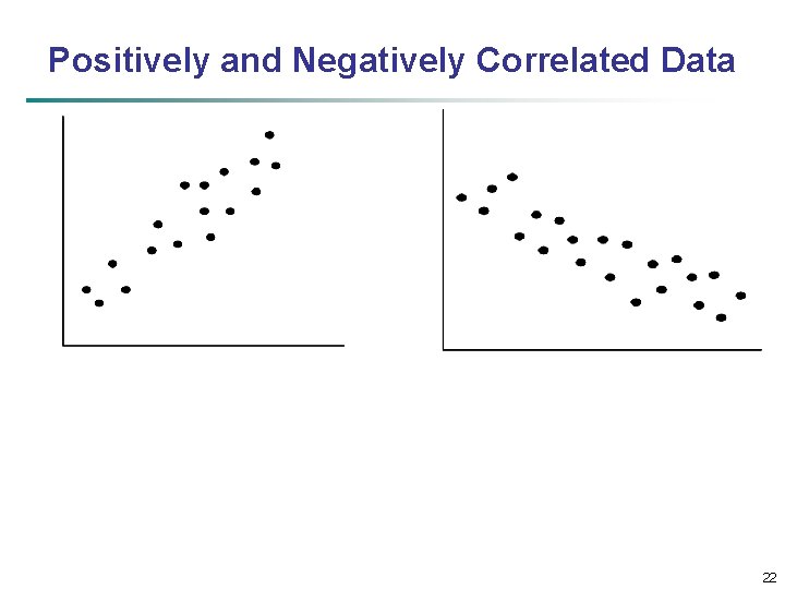
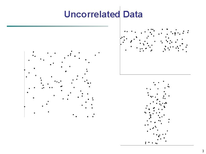
Graphic Displays of Basic Statistical Descriptions n Boxplot: graphic display of five-number summary n Histogram: x-axis are values, y-axis represents frequencies n Quantile plot: each value xi is paired with fi indicating that approximately fi * 100% of data are below the value xi n Quantile-quantile (q-q) plot: graphs the quantiles of one univariant distribution against the corresponding quantiles of another n Scatter plot: each pair of values is a pair of coordinates and plotted as points in the plane 17

Histogram Example 18

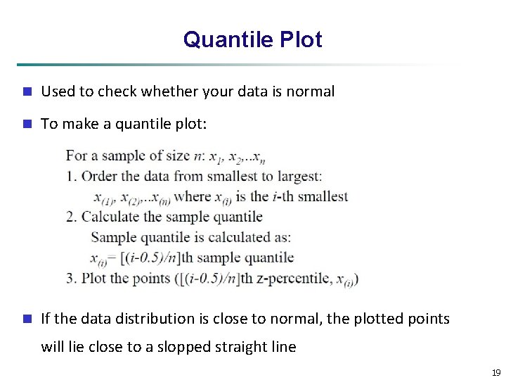
Quantile Plot n Used to check whether your data is normal n To make a quantile plot: n If the data distribution is close to normal, the plotted points will lie close to a slopped straight line 19

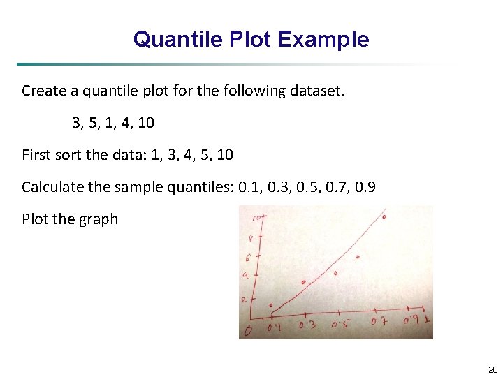
Quantile Plot Example Create a quantile plot for the following dataset. 3, 5, 1, 4, 10 First sort the data: 1, 3, 4, 5, 10 Calculate the sample quantiles: 0. 1, 0. 3, 0. 5, 0. 7, 0. 9 Plot the graph 20

Scatter Plot 21

Positively and Negatively Correlated Data 22

Uncorrelated Data 23

Chapter 2: Getting to Know Your Data n Data Objects and Attribute Types n Basic Statistical Descriptions of Data n Data Visualization n Measuring Data Similarity and Dissimilarity n Summary 24

Data Visualization n n Why data visualization? n Gain insight into the data n Search for patterns, trends, structure, irregularities, relationships among data Categorization of visualization methods: n Pixel-oriented visualization techniques n Geometric projection visualization techniques n Icon-based visualization techniques n Hierarchical visualization techniques n Visualizing complex data and relations 25

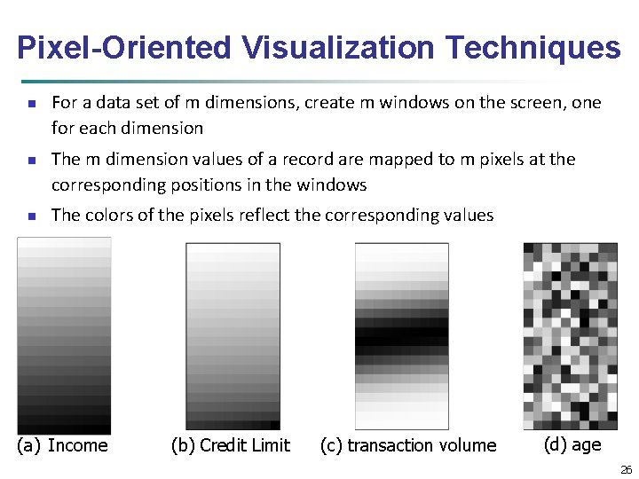
Pixel-Oriented Visualization Techniques n n n For a data set of m dimensions, create m windows on the screen, one for each dimension The m dimension values of a record are mapped to m pixels at the corresponding positions in the windows The colors of the pixels reflect the corresponding values (a) Income (b) Credit Limit (c) transaction volume (d) age 26

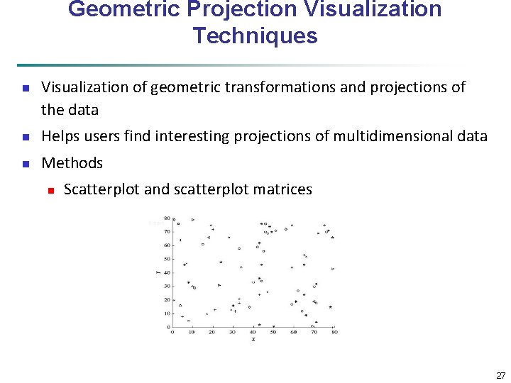
Geometric Projection Visualization Techniques n Visualization of geometric transformations and projections of the data n Helps users find interesting projections of multidimensional data n Methods n Scatterplot and scatterplot matrices 27

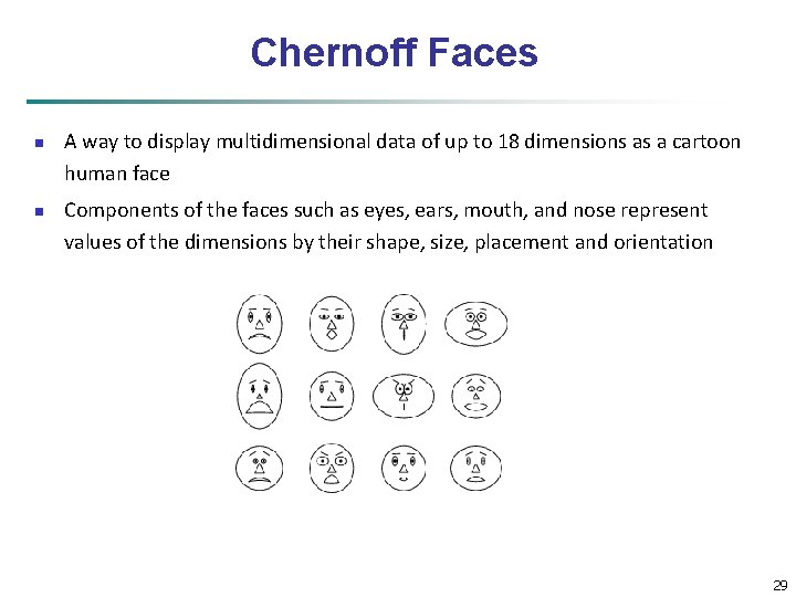
Icon-Based Visualization Techniques n Visualization of the data values as features of icons n Typical visualization methods n Chernoff Faces n Stick Figures 28

Chernoff Faces n n A way to display multidimensional data of up to 18 dimensions as a cartoon human face Components of the faces such as eyes, ears, mouth, and nose represent values of the dimensions by their shape, size, placement and orientation 29

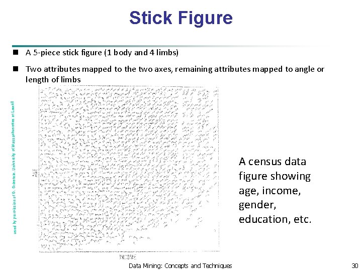
Stick Figure n A 5 -piece stick figure (1 body and 4 limbs) used by permission of G. Grinstein, University of Massachusettes at Lowell n Two attributes mapped to the two axes, remaining attributes mapped to angle or length of limbs A census data figure showing age, income, gender, education, etc. Data Mining: Concepts and Techniques 30

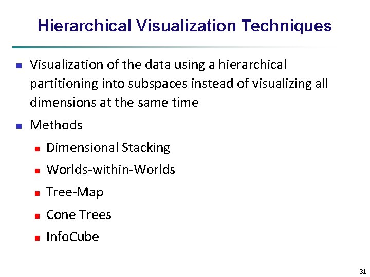
Hierarchical Visualization Techniques n n Visualization of the data using a hierarchical partitioning into subspaces instead of visualizing all dimensions at the same time Methods n Dimensional Stacking n Worlds-within-Worlds n Tree-Map n Cone Trees n Info. Cube 31

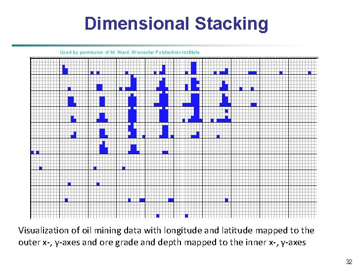
Dimensional Stacking Used by permission of M. Ward, Worcester Polytechnic Institute Visualization of oil mining data with longitude and latitude mapped to the outer x-, y-axes and ore grade and depth mapped to the inner x-, y-axes 32

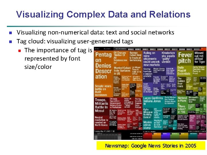
Visualizing Complex Data and Relations n n Visualizing non-numerical data: text and social networks Tag cloud: visualizing user-generated tags n The importance of tag is represented by font size/color Newsmap: Google News Stories in 2005

Chapter 2: Getting to Know Your Data n Data Objects and Attribute Types n Basic Statistical Descriptions of Data n Data Visualization n Measuring Data Similarity and Dissimilarity n Summary 34

Similarity and Dissimilarity n n n Similarity n Numerical measure of how alike two data objects are n Value is higher when objects are more alike n Often falls in the range [0, 1] Dissimilarity n Numerical measure of how different two data objects are n Lower when objects are more alike Two data structures commonly used to measure the above n Data matrix n Dissimilarity matrix 35

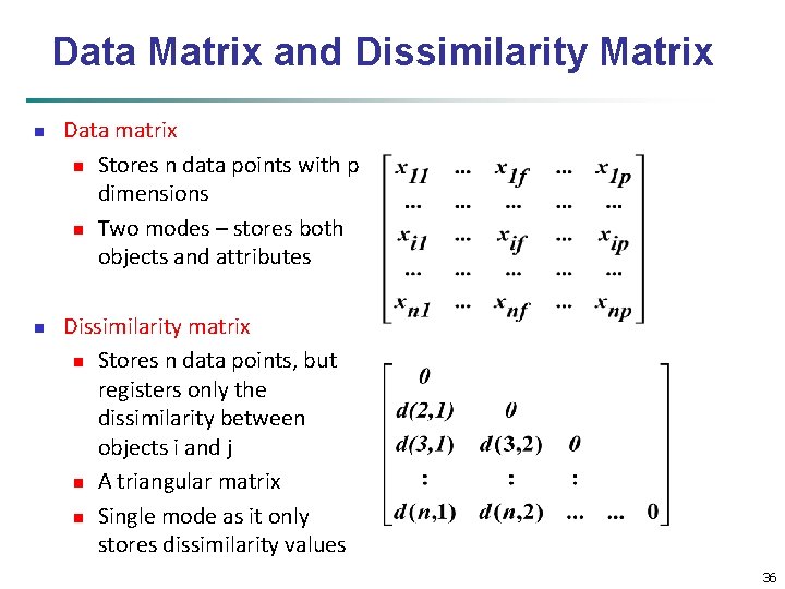
Data Matrix and Dissimilarity Matrix n n Data matrix n Stores n data points with p dimensions n Two modes – stores both objects and attributes Dissimilarity matrix n Stores n data points, but registers only the dissimilarity between objects i and j n A triangular matrix n Single mode as it only stores dissimilarity values 36

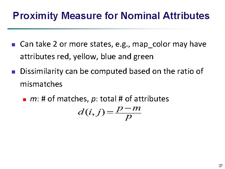
Proximity Measure for Nominal Attributes n n Can take 2 or more states, e. g. , map_color may have attributes red, yellow, blue and green Dissimilarity can be computed based on the ratio of mismatches n m: # of matches, p: total # of attributes 37

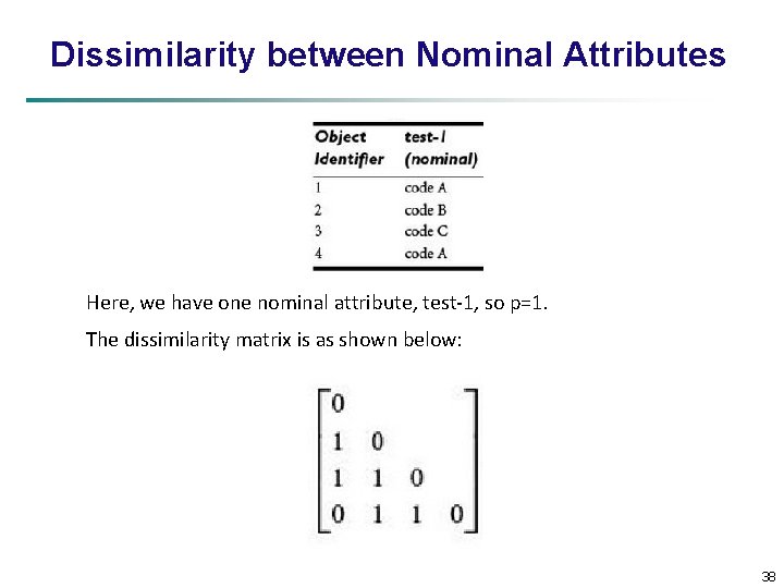
Dissimilarity between Nominal Attributes Here, we have one nominal attribute, test-1, so p=1. The dissimilarity matrix is as shown below: 38

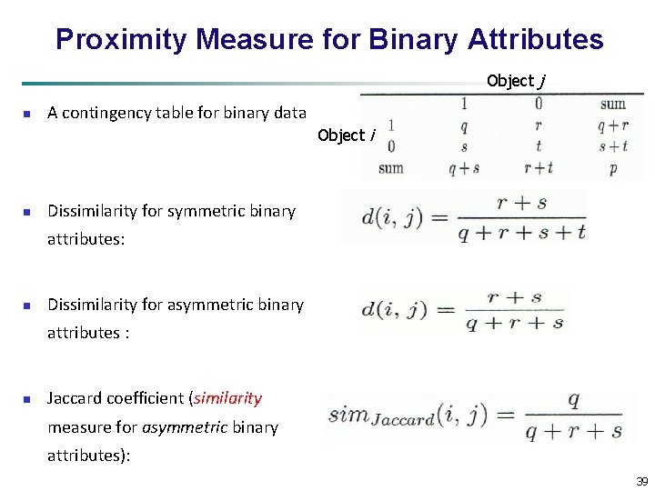
Proximity Measure for Binary Attributes Object j n A contingency table for binary data Object i n Dissimilarity for symmetric binary attributes: n Dissimilarity for asymmetric binary attributes : n Jaccard coefficient (similarity measure for asymmetric binary attributes): 39

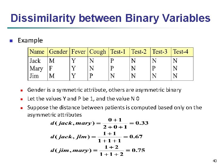
Dissimilarity between Binary Variables n Example n n n Gender is a symmetric attribute, others are asymmetric binary Let the values Y and P be 1, and the value N 0 Suppose the distance between patients is computed based only on the asymmetric attributes 40

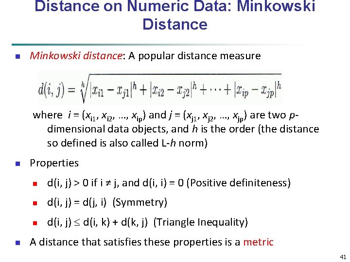
Distance on Numeric Data: Minkowski Distance n Minkowski distance: A popular distance measure where i = (xi 1, xi 2, …, xip) and j = (xj 1, xj 2, …, xjp) are two pdimensional data objects, and h is the order (the distance so defined is also called L-h norm) n n Properties n d(i, j) > 0 if i ≠ j, and d(i, i) = 0 (Positive definiteness) n d(i, j) = d(j, i) (Symmetry) n d(i, j) d(i, k) + d(k, j) (Triangle Inequality) A distance that satisfies these properties is a metric 41

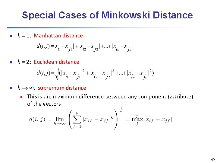
Special Cases of Minkowski Distance n h = 1: Manhattan distance n h = 2: Euclidean distance n h . supremum distance n This is the maximum difference between any component (attribute) of the vectors 42

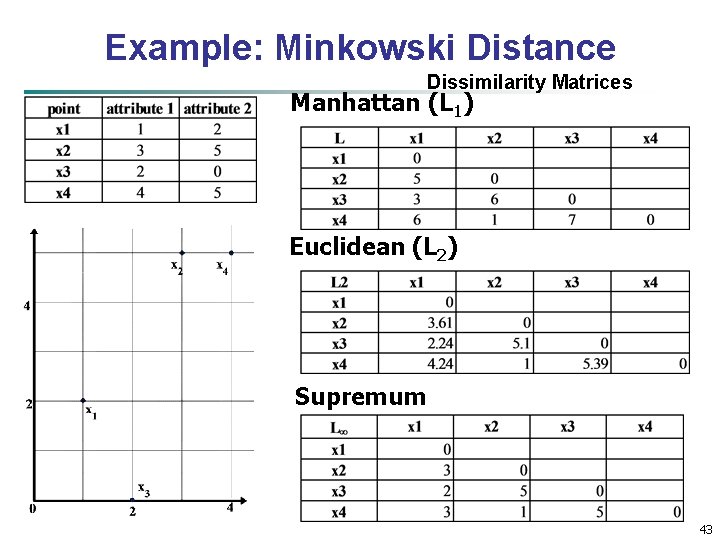
Example: Minkowski Distance Dissimilarity Matrices Manhattan (L 1) Euclidean (L 2) Supremum 43

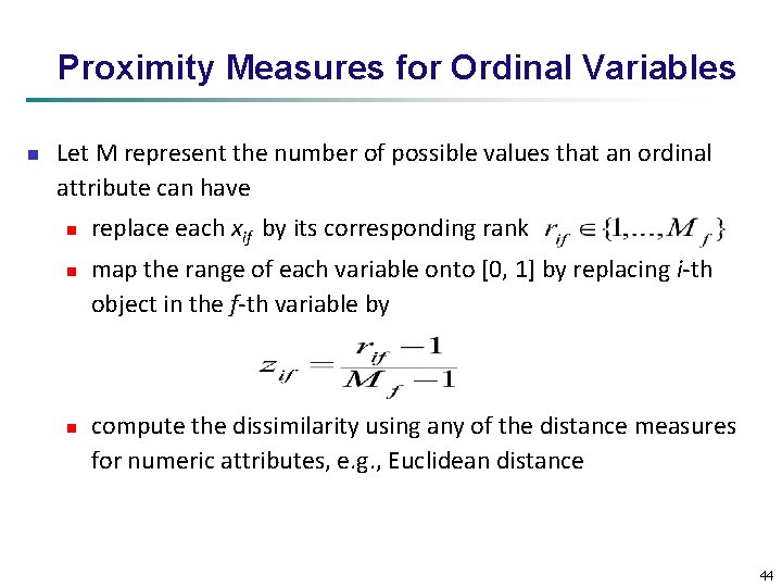
Proximity Measures for Ordinal Variables n Let M represent the number of possible values that an ordinal attribute can have n n n replace each xif by its corresponding rank map the range of each variable onto [0, 1] by replacing i-th object in the f-th variable by compute the dissimilarity using any of the distance measures for numeric attributes, e. g. , Euclidean distance 44

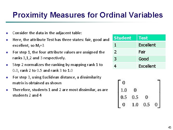
Proximity Measures for Ordinal Variables n n n Consider the data in the adjacent table: Here, the attribute Test has three states: fair, good and excellent, so Mf=3 Student Test 1 Excellent For step 1, the four attribute values are assigned the ranks 3, 1, 2 and 3 respectively. 2 Fair 3 Good Step 2 normalizes the ranking by mapping rank 1 to 0. 0, rank 2 to 0. 5 and rank 3 to 1. 0 4 Excellent For step 3, using Euclidean distance, a dissimilarity matrix is obtained as shown Therefore, students 1 and 2 are most dissimilar, as are students 2 and 4 45

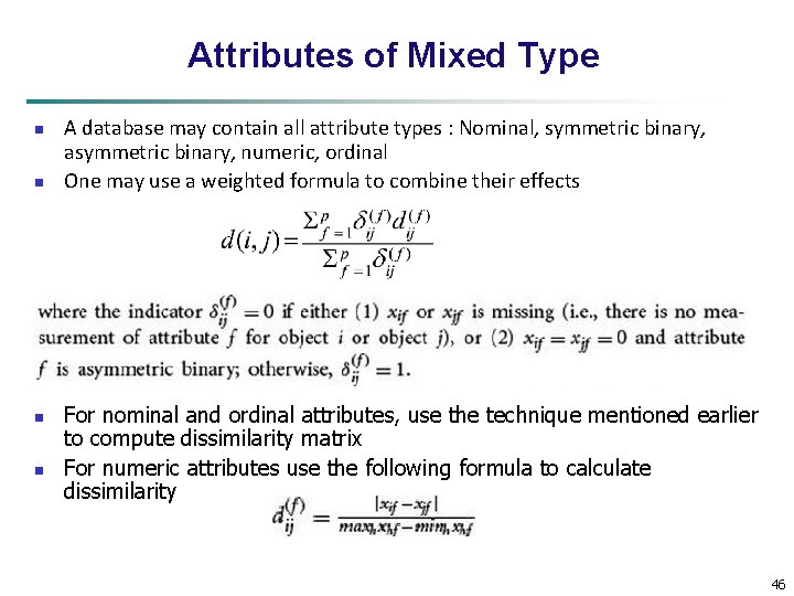
Attributes of Mixed Type n n A database may contain all attribute types : Nominal, symmetric binary, asymmetric binary, numeric, ordinal One may use a weighted formula to combine their effects For nominal and ordinal attributes, use the technique mentioned earlier to compute dissimilarity matrix For numeric attributes use the following formula to calculate dissimilarity 46

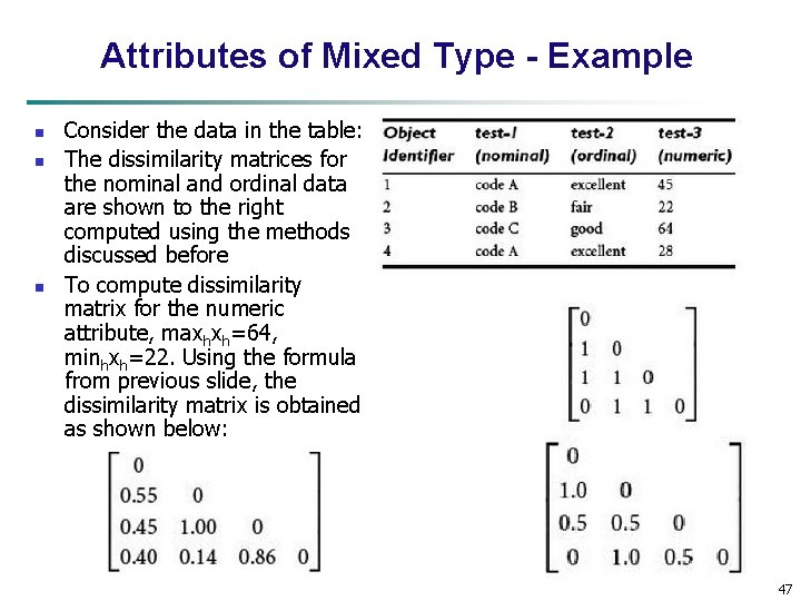
Attributes of Mixed Type - Example n n n Consider the data in the table: The dissimilarity matrices for the nominal and ordinal data are shown to the right computed using the methods discussed before To compute dissimilarity matrix for the numeric attribute, maxhxh=64, minhxh=22. Using the formula from previous slide, the dissimilarity matrix is obtained as shown below: 47

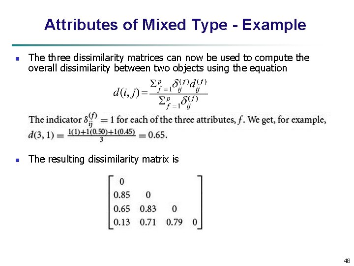
Attributes of Mixed Type - Example n n The three dissimilarity matrices can now be used to compute the overall dissimilarity between two objects using the equation The resulting dissimilarity matrix is 48

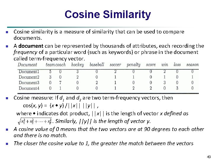
Cosine Similarity n n n Cosine similarity is a measure of similarity that can be used to compare documents. A document can be represented by thousands of attributes, each recording the frequency of a particular word (such as keywords) or phrase in the document called term-frequency vector. Cosine measure: If d 1 and d 2 are two term-frequency vectors, then cos(x, y) = (x y) /||x|| ||y|| , where indicates dot product, ||x|| is the length of vector x defined as. Similarly, ||y|| is the length of vector y. A cosine value of 0 means that the two vectors are at 90 degrees to each other and there is no match. The closer the cosine value to 1, the greater the match between the vectors 49

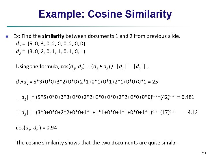
Example: Cosine Similarity n Ex: Find the similarity between documents 1 and 2 from previous slide. d 1 = (5, 0, 3, 0, 2, 0, 0) d 2 = (3, 0, 2, 0, 1, 1, 0, 1) Using the formula, cos(d 1, d 2) = (d 1 d 2) /||d 1|| ||d 2|| , d 1 d 2 = 5*3+0*0+3*2+0*0+2*1+0*1+2*1+0*0+0*1 = 25 ||d 1||= (5*5+0*0+3*3+0*0+2*2+0*0+0*0)0. 5=(42)0. 5 = 6. 481 ||d 2||= (3*3+0*0+2*2+0*0+1*1+0*0+1*1)0. 5=(17)0. 5 = 4. 12 cos(d 1, d 2 ) = 0. 94 The cosine similarity shows that the two documents are quite similar. 50

Chapter 2: Getting to Know Your Data n Data Objects and Attribute Types n Basic Statistical Descriptions of Data n Data Visualization n Measuring Data Similarity and Dissimilarity n Summary 51

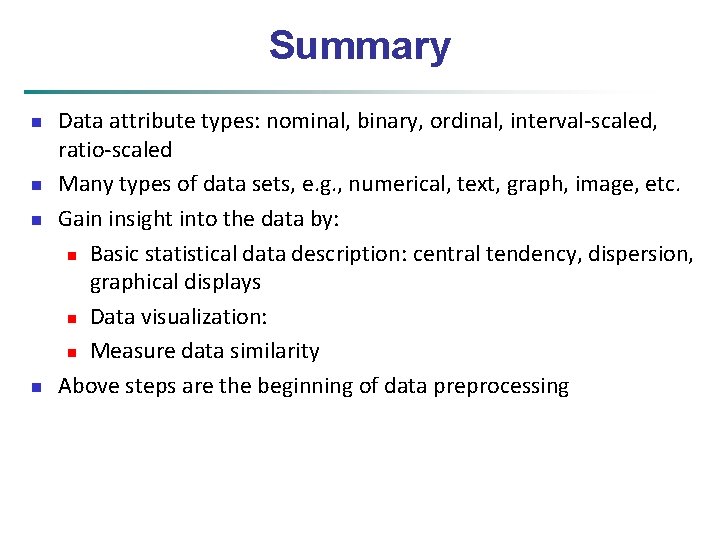
Summary n n Data attribute types: nominal, binary, ordinal, interval-scaled, ratio-scaled Many types of data sets, e. g. , numerical, text, graph, image, etc. Gain insight into the data by: n Basic statistical data description: central tendency, dispersion, graphical displays n Data visualization: n Measure data similarity Above steps are the beginning of data preprocessing

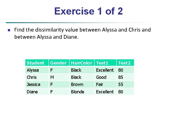
Exercise 1 of 2 n Find the dissimilarity value between Alyssa and Chris and between Alyssa and Diane. Student Gender Hair. Color Test 1 Test 2 Alyssa F Black Excellent 80 Chris M Black Good 85 Jessica F Brown Fair 55 Diane F Blonde Excellent 80

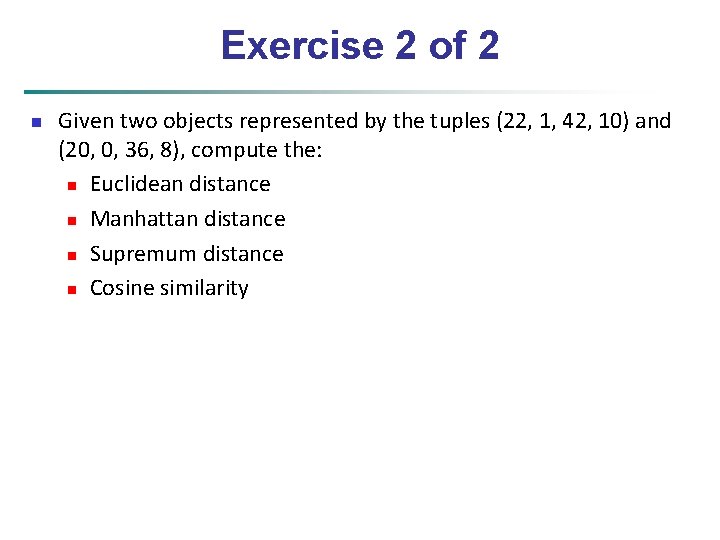
Exercise 2 of 2 n Given two objects represented by the tuples (22, 1, 42, 10) and (20, 0, 36, 8), compute the: n Euclidean distance n Manhattan distance n Supremum distance n Cosine similarity