Data Mining Concepts and Techniques Chapter 2 Getting

Data Mining: Concepts and Techniques — Chapter 2 — (Getting to Know Your Data) Jiawei Han, Micheline Kamber, and Jian Pei University of Illinois at Urbana-Champaign Simon Fraser University © 2011 Han, Kamber, and Pei. All rights reserved. 1

Chapter 2: Getting to Know Your Data n Data Objects and Attribute Types n Basic Statistical Descriptions of Data n Data Visualization n Measuring Data Similarity and Dissimilarity n Summary 2

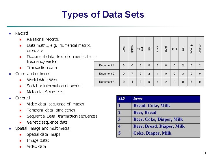
Types of Data Sets n n Record n Relational records n Data matrix, e. g. , numerical matrix, crosstabs n Document data: text documents: termfrequency vector n Transaction data Graph and network n World Wide Web n Social or information networks n Molecular Structures Ordered n Video data: sequence of images n Temporal data: time-series n Sequential Data: transaction sequences n Genetic sequence data Spatial, image and multimedia: n Spatial data: maps n Image data: n Video data: 3

Important Characteristics of Structured Data n Dimensionality n n Sparsity n n Only presence counts Resolution n n Curse of dimensionality Patterns depend on the scale Distribution n Centrality and dispersion 4

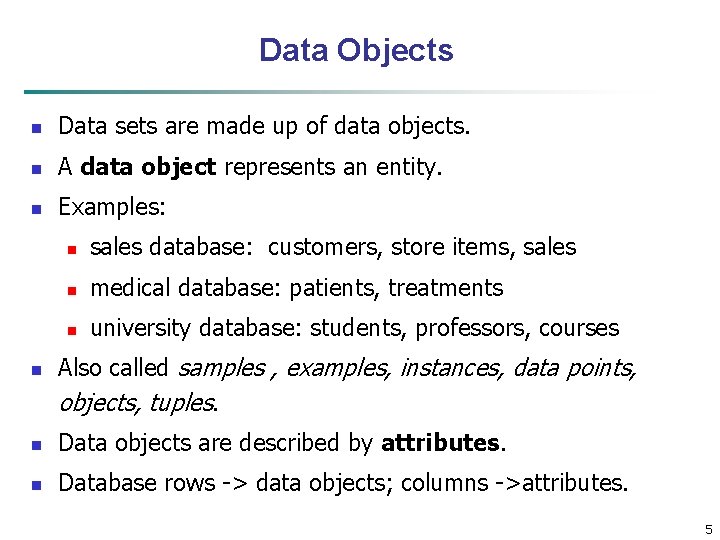
Data Objects n Data sets are made up of data objects. n A data object represents an entity. n Examples: n n sales database: customers, store items, sales n medical database: patients, treatments n university database: students, professors, courses Also called samples , examples, instances, data points, objects, tuples. n Data objects are described by attributes. n Database rows -> data objects; columns ->attributes. 5

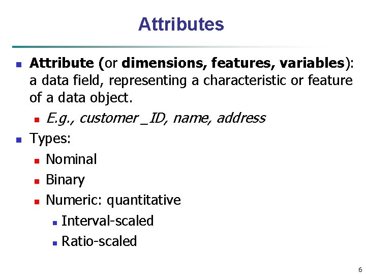
Attributes n Attribute (or dimensions, features, variables): a data field, representing a characteristic or feature of a data object. n n E. g. , customer _ID, name, address Types: n Nominal n Binary n Numeric: quantitative n Interval-scaled n Ratio-scaled 6

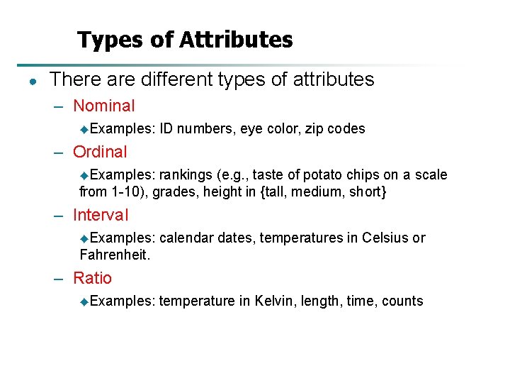
Types of Attributes ● There are different types of attributes – Nominal ◆Examples: ID numbers, eye color, zip codes – Ordinal ◆Examples: rankings (e. g. , taste of potato chips on a scale from 1 -10), grades, height in {tall, medium, short} – Interval ◆Examples: calendar dates, temperatures in Celsius or Fahrenheit. – Ratio ◆Examples: temperature in Kelvin, length, time, counts

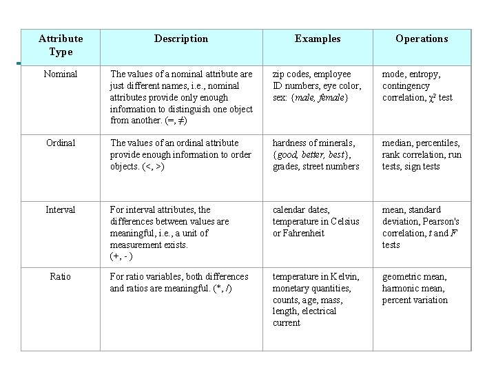
Attribute Type Description Examples Nominal The values of a nominal attribute are just different names, i. e. , nominal attributes provide only enough information to distinguish one object from another. (=, ≠) zip codes, employee ID numbers, eye color, sex: {male, female} mode, entropy, contingency correlation, χ2 test Ordinal The values of an ordinal attribute provide enough information to order objects. (<, >) hardness of minerals, {good, better, best}, grades, street numbers median, percentiles, rank correlation, run tests, sign tests Interval For interval attributes, the differences between values are meaningful, i. e. , a unit of measurement exists. (+, - ) calendar dates, temperature in Celsius or Fahrenheit mean, standard deviation, Pearson's correlation, t and F tests For ratio variables, both differences and ratios are meaningful. (*, /) temperature in Kelvin, monetary quantities, counts, age, mass, length, electrical current geometric mean, harmonic mean, percent variation Ratio Operations

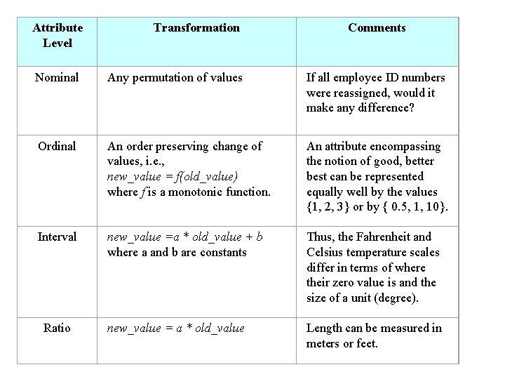
Attribute Level Transformation Nominal Any permutation of values If all employee ID numbers were reassigned, would it make any difference? Ordinal An order preserving change of values, i. e. , new_value = f(old_value) where f is a monotonic function. An attribute encompassing the notion of good, better best can be represented equally well by the values {1, 2, 3} or by { 0. 5, 1, 10}. Interval new_value =a * old_value + b where a and b are constants Thus, the Fahrenheit and Celsius temperature scales differ in terms of where their zero value is and the size of a unit (degree). new_value = a * old_value Length can be measured in meters or feet. Ratio Comments

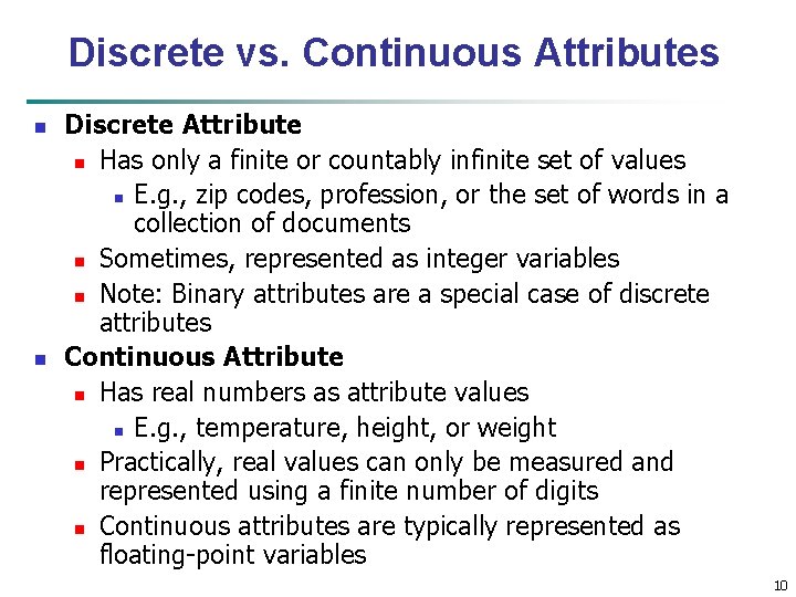
Discrete vs. Continuous Attributes n n Discrete Attribute n Has only a finite or countably infinite set of values n E. g. , zip codes, profession, or the set of words in a collection of documents n Sometimes, represented as integer variables n Note: Binary attributes are a special case of discrete attributes Continuous Attribute n Has real numbers as attribute values n E. g. , temperature, height, or weight n Practically, real values can only be measured and represented using a finite number of digits n Continuous attributes are typically represented as floating-point variables 10

Chapter 2: Getting to Know Your Data n Data Objects and Attribute Types n Basic Statistical Descriptions of Data n Data Visualization n Measuring Data Similarity and Dissimilarity n Summary 11

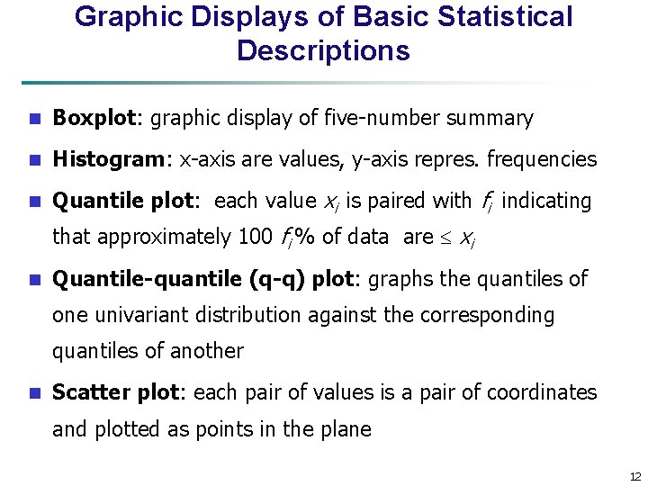
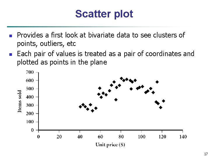
Graphic Displays of Basic Statistical Descriptions n Boxplot: graphic display of five-number summary n Histogram: x-axis are values, y-axis repres. frequencies n Quantile plot: each value xi is paired with fi indicating that approximately 100 fi % of data are xi n Quantile-quantile (q-q) plot: graphs the quantiles of one univariant distribution against the corresponding quantiles of another n Scatter plot: each pair of values is a pair of coordinates and plotted as points in the plane 12

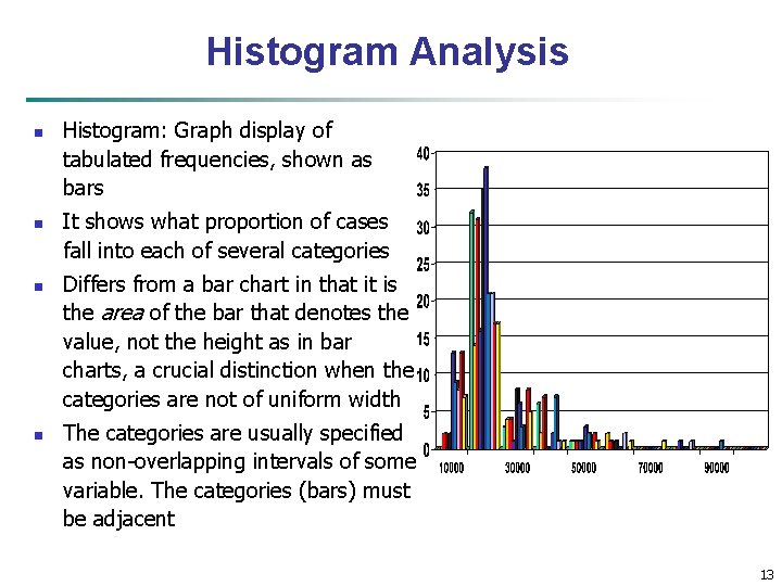
Histogram Analysis n n Histogram: Graph display of tabulated frequencies, shown as bars It shows what proportion of cases fall into each of several categories Differs from a bar chart in that it is the area of the bar that denotes the value, not the height as in bar charts, a crucial distinction when the categories are not of uniform width The categories are usually specified as non-overlapping intervals of some variable. The categories (bars) must be adjacent 13

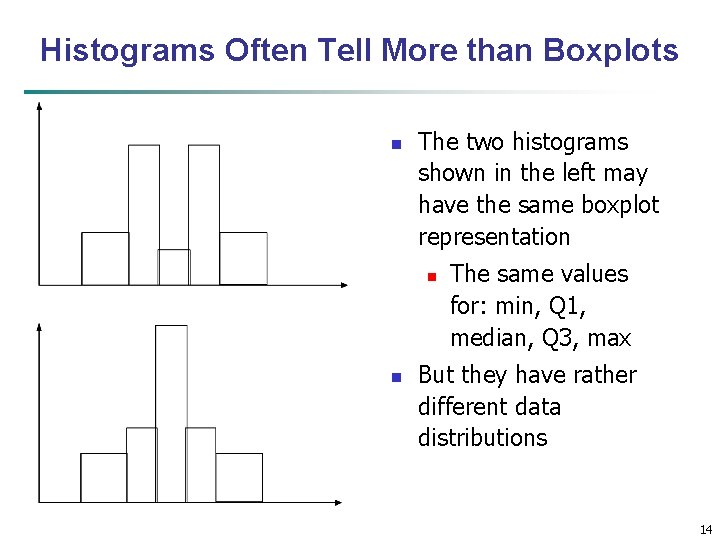
Histograms Often Tell More than Boxplots n The two histograms shown in the left may have the same boxplot representation n n The same values for: min, Q 1, median, Q 3, max But they have rather different data distributions 14

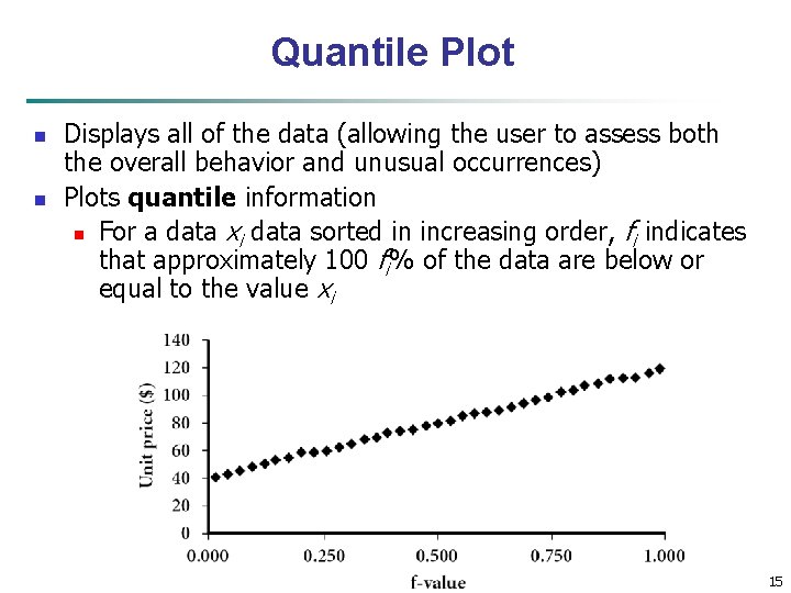
Quantile Plot n n Displays all of the data (allowing the user to assess both the overall behavior and unusual occurrences) Plots quantile information n For a data xi data sorted in increasing order, fi indicates that approximately 100 fi% of the data are below or equal to the value xi Data Mining: Concepts and Techniques 15

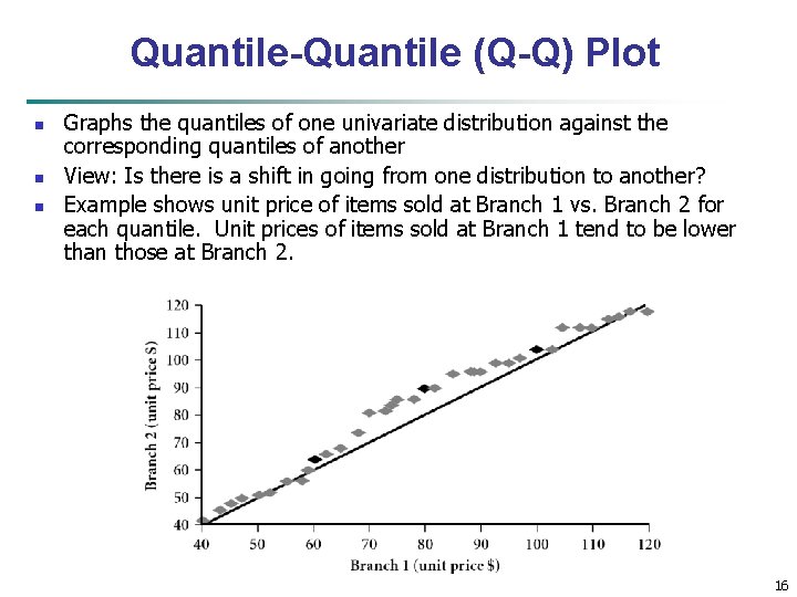
Quantile-Quantile (Q-Q) Plot n n n Graphs the quantiles of one univariate distribution against the corresponding quantiles of another View: Is there is a shift in going from one distribution to another? Example shows unit price of items sold at Branch 1 vs. Branch 2 for each quantile. Unit prices of items sold at Branch 1 tend to be lower than those at Branch 2. 16

Scatter plot n n Provides a first look at bivariate data to see clusters of points, outliers, etc Each pair of values is treated as a pair of coordinates and plotted as points in the plane 17

Chapter 2: Getting to Know Your Data n Data Objects and Attribute Types n Basic Statistical Descriptions of Data n Data Visualization n Measuring Data Similarity and Dissimilarity n Summary 18

Data Visualization n Why data visualization? n n n Gain insight into an information space by mapping data onto graphical primitives Provide qualitative overview of large data sets Search for patterns, trends, structure, irregularities, relationships among data Help find interesting regions and suitable parameters for further quantitative analysis Provide a visual proof of computer representations derived Categorization of visualization methods: n Pixel-oriented visualization techniques n Geometric projection visualization techniques n Icon-based visualization techniques n Hierarchical visualization techniques n Visualizing complex data and relations 19

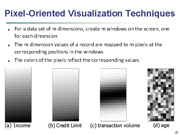
Pixel-Oriented Visualization Techniques ■ ■ ■ For a data set of m dimensions, create m windows on the screen, one for each dimension The m dimension values of a record are mapped to m pixels at the corresponding positions in the windows The colors of the pixels reflect the corresponding values (a) Income (b) Credit Limit (c) transaction volume (d) age 20

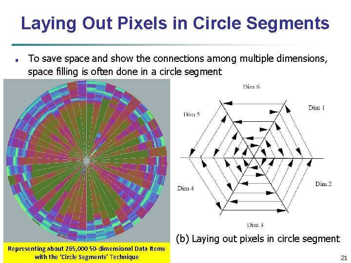
Laying Out Pixels in Circle Segments ■ To save space and show the connections among multiple dimensions, space filling is often done in a circle segment (a) Representing a data record circle segment. Data Items Representing aboutin 265, 000 50 -dimensional with the ‘Circle Segments’ Technique (b) Laying out pixels in circle segment 21

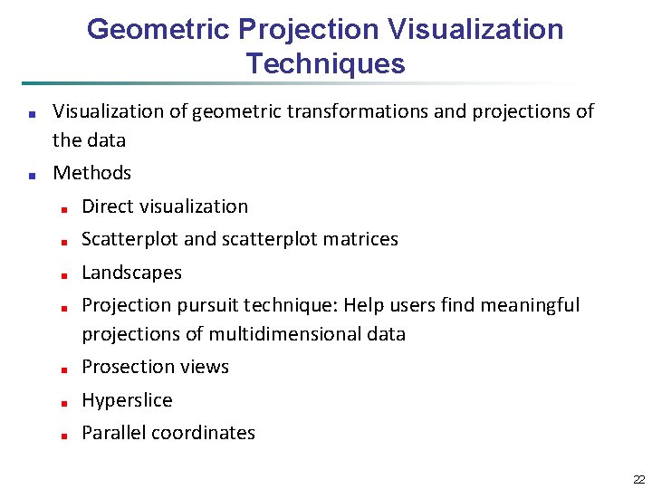
Geometric Projection Visualization Techniques ■ ■ Visualization of geometric transformations and projections of the data Methods ■ Direct visualization ■ Scatterplot and scatterplot matrices ■ Landscapes ■ Projection pursuit technique: Help users find meaningful projections of multidimensional data ■ Prosection views ■ Hyperslice ■ Parallel coordinates 22

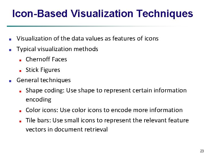
Icon-Based Visualization Techniques ■ Visualization of the data values as features of icons ■ Typical visualization methods ■ ■ Chernoff Faces ■ Stick Figures General techniques ■ ■ ■ Shape coding: Use shape to represent certain information encoding Color icons: Use color icons to encode more information Tile bars: Use small icons to represent the relevant feature vectors in document retrieval 23

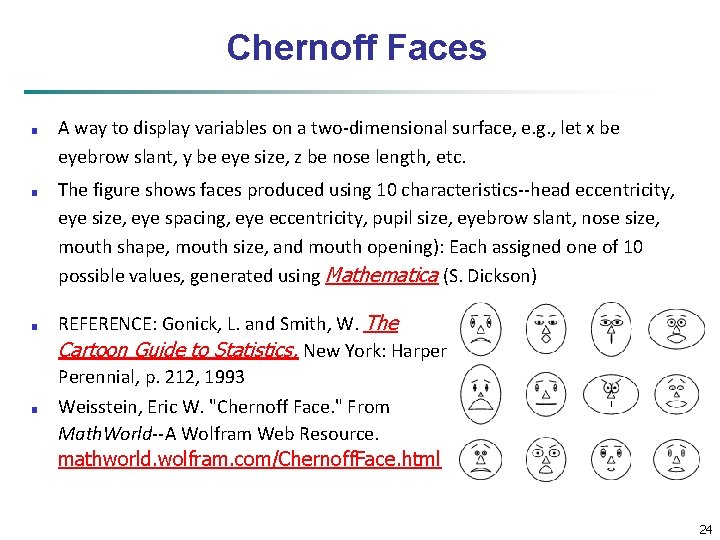
Chernoff Faces ■ ■ A way to display variables on a two-dimensional surface, e. g. , let x be eyebrow slant, y be eye size, z be nose length, etc. The figure shows faces produced using 10 characteristics--head eccentricity, eye size, eye spacing, eye eccentricity, pupil size, eyebrow slant, nose size, mouth shape, mouth size, and mouth opening): Each assigned one of 10 possible values, generated using Mathematica (S. Dickson) REFERENCE: Gonick, L. and Smith, W. The Cartoon Guide to Statistics. New York: Harper Perennial, p. 212, 1993 Weisstein, Eric W. "Chernoff Face. " From Math. World--A Wolfram Web Resource. mathworld. wolfram. com/Chernoff. Face. html 24

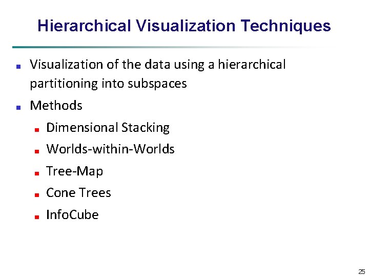
Hierarchical Visualization Techniques ■ ■ Visualization of the data using a hierarchical partitioning into subspaces Methods ■ Dimensional Stacking ■ Worlds-within-Worlds ■ Tree-Map ■ Cone Trees ■ Info. Cube 25

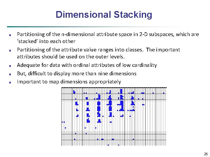
Dimensional Stacking ■ ■ ■ Partitioning of the n-dimensional attribute space in 2 -D subspaces, which are ‘stacked’ into each other Partitioning of the attribute value ranges into classes. The important attributes should be used on the outer levels. Adequate for data with ordinal attributes of low cardinality But, difficult to display more than nine dimensions Important to map dimensions appropriately 26

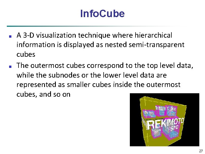
Info. Cube ■ ■ A 3 -D visualization technique where hierarchical information is displayed as nested semi-transparent cubes The outermost cubes correspond to the top level data, while the subnodes or the lower level data are represented as smaller cubes inside the outermost cubes, and so on 27

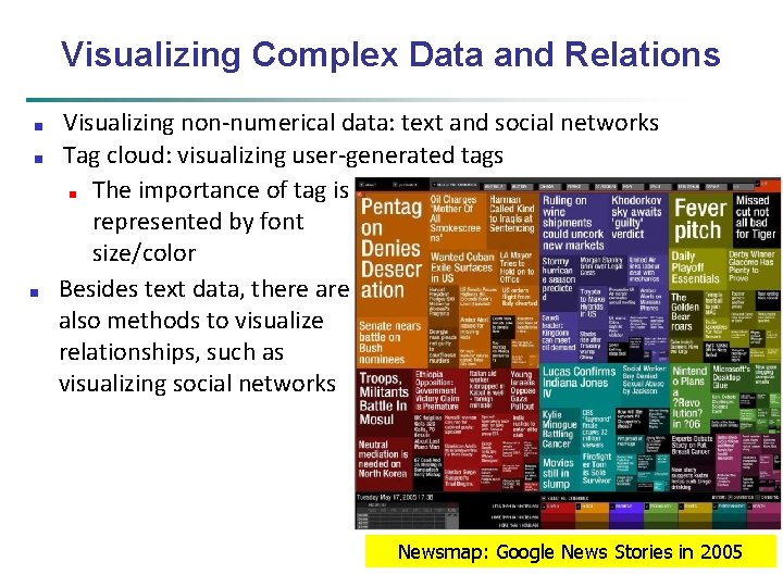
Visualizing Complex Data and Relations ■ ■ ■ Visualizing non-numerical data: text and social networks Tag cloud: visualizing user-generated tags ■ The importance of tag is represented by font size/color Besides text data, there also methods to visualize relationships, such as visualizing social networks Newsmap: Google News Stories in 2005

Chapter 2: Getting to Know Your Data n Data Objects and Attribute Types n Basic Statistical Descriptions of Data n Data Visualization n Measuring Data Similarity and Dissimilarity n Summary 29

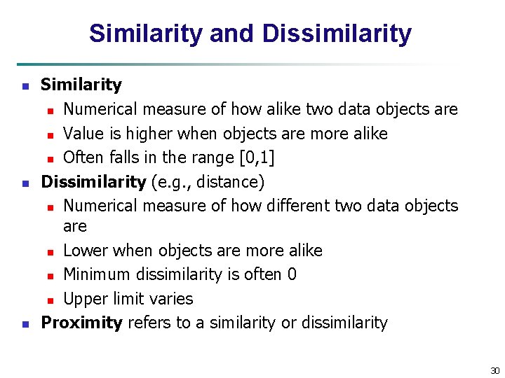
Similarity and Dissimilarity n n n Similarity n Numerical measure of how alike two data objects are n Value is higher when objects are more alike n Often falls in the range [0, 1] Dissimilarity (e. g. , distance) n Numerical measure of how different two data objects are n Lower when objects are more alike n Minimum dissimilarity is often 0 n Upper limit varies Proximity refers to a similarity or dissimilarity 30

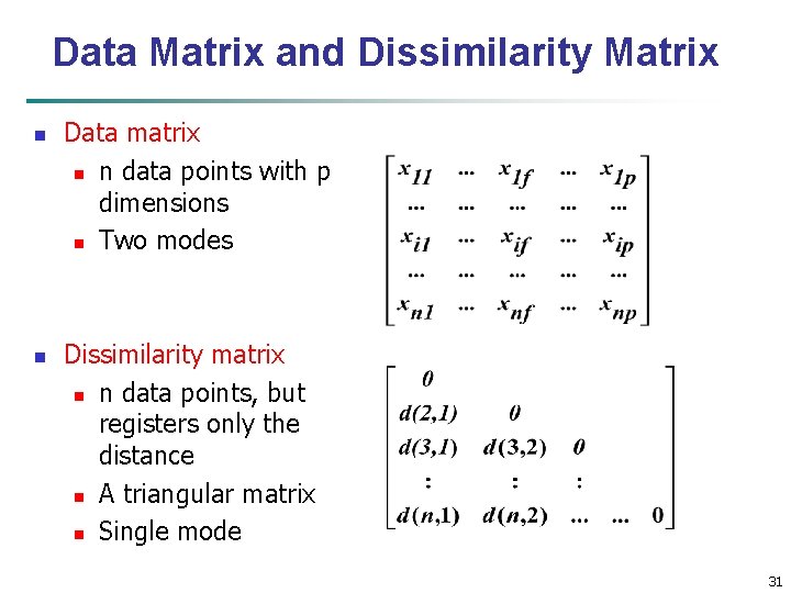
Data Matrix and Dissimilarity Matrix n n Data matrix n n data points with p dimensions n Two modes Dissimilarity matrix n n data points, but registers only the distance n A triangular matrix n Single mode 31

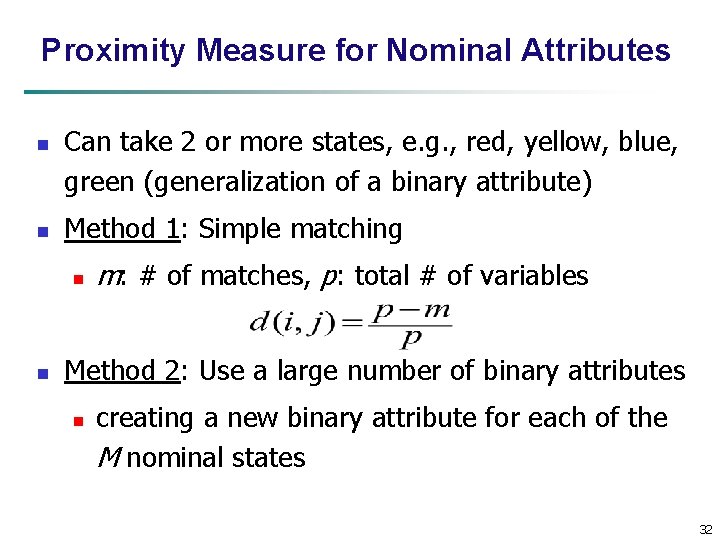
Proximity Measure for Nominal Attributes n n Can take 2 or more states, e. g. , red, yellow, blue, green (generalization of a binary attribute) Method 1: Simple matching n n m: # of matches, p: total # of variables Method 2: Use a large number of binary attributes n creating a new binary attribute for each of the M nominal states 32

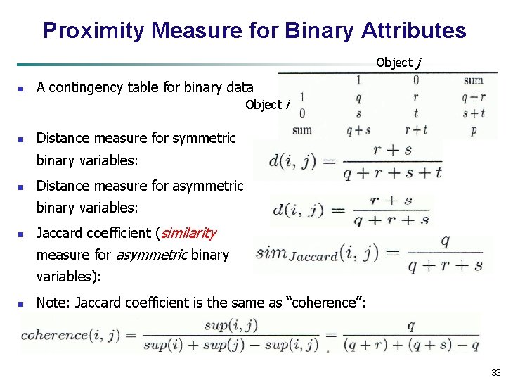
Proximity Measure for Binary Attributes Object j n A contingency table for binary data Object i n Distance measure for symmetric binary variables: n Distance measure for asymmetric binary variables: n Jaccard coefficient (similarity measure for asymmetric binary variables): n Note: Jaccard coefficient is the same as “coherence”: 33

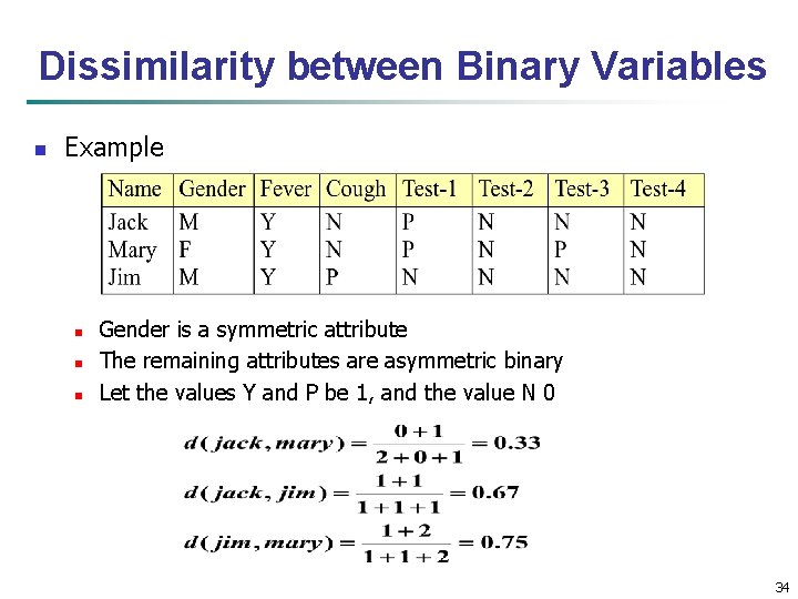
Dissimilarity between Binary Variables n Example n n n Gender is a symmetric attribute The remaining attributes are asymmetric binary Let the values Y and P be 1, and the value N 0 34

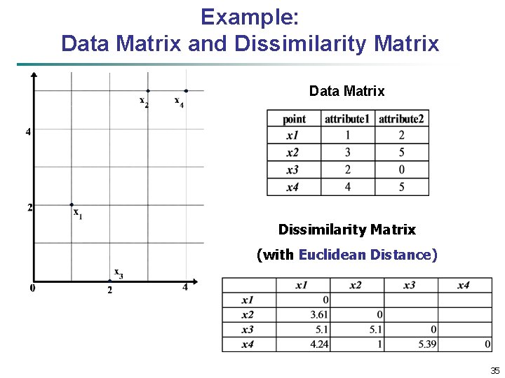
Example: Data Matrix and Dissimilarity Matrix Data Matrix Dissimilarity Matrix (with Euclidean Distance) 35

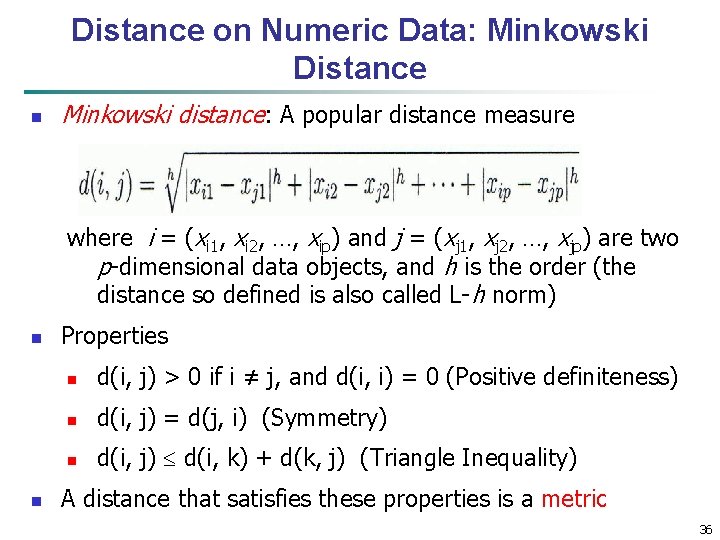
Distance on Numeric Data: Minkowski Distance n Minkowski distance: A popular distance measure where i = (xi 1, xi 2, …, xip) and j = (xj 1, xj 2, …, xjp) are two p-dimensional data objects, and h is the order (the distance so defined is also called L-h norm) n n Properties n d(i, j) > 0 if i ≠ j, and d(i, i) = 0 (Positive definiteness) n d(i, j) = d(j, i) (Symmetry) n d(i, j) d(i, k) + d(k, j) (Triangle Inequality) A distance that satisfies these properties is a metric 36

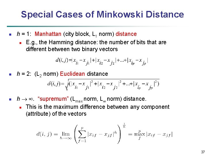
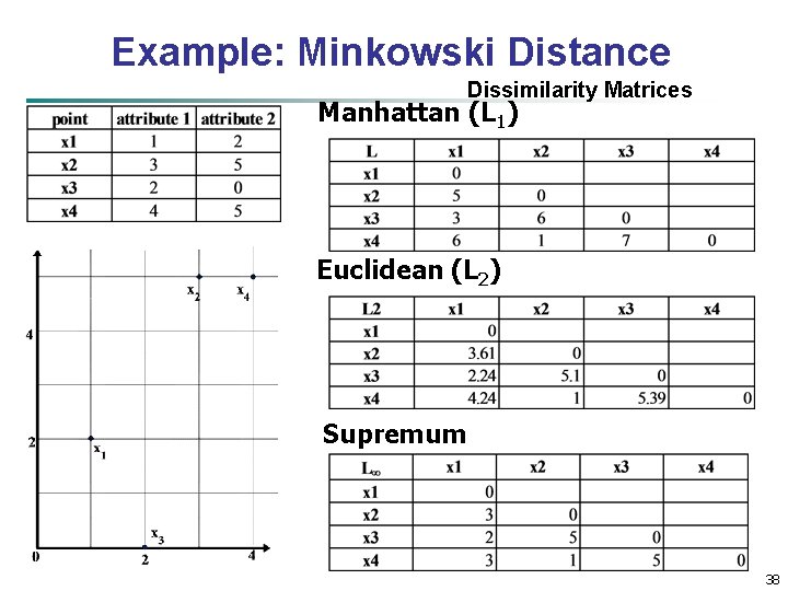
Special Cases of Minkowski Distance n n n h = 1: Manhattan (city block, L 1 norm) distance n E. g. , the Hamming distance: the number of bits that are different between two binary vectors h = 2: (L 2 norm) Euclidean distance h . “supremum” (Lmax norm, L norm) distance. n This is the maximum difference between any component (attribute) of the vectors 37

Example: Minkowski Distance Dissimilarity Matrices Manhattan (L 1) Euclidean (L 2) Supremum 38

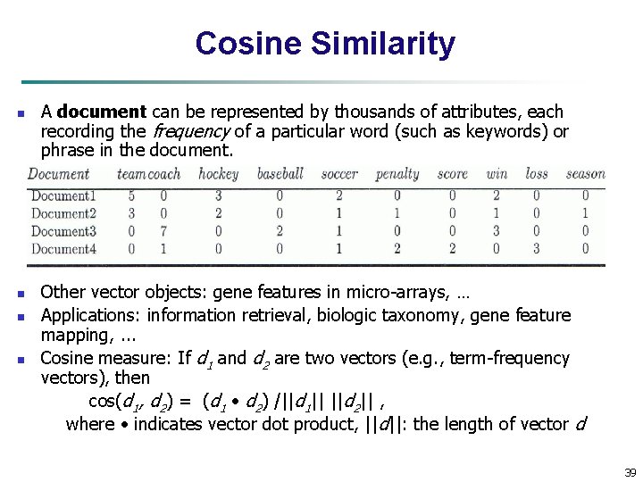
Cosine Similarity n n A document can be represented by thousands of attributes, each recording the frequency of a particular word (such as keywords) or phrase in the document. Other vector objects: gene features in micro-arrays, … Applications: information retrieval, biologic taxonomy, gene feature mapping, . . . Cosine measure: If d 1 and d 2 are two vectors (e. g. , term-frequency vectors), then cos(d 1, d 2) = (d 1 d 2) /||d 1|| ||d 2|| , where indicates vector dot product, ||d||: the length of vector d 39

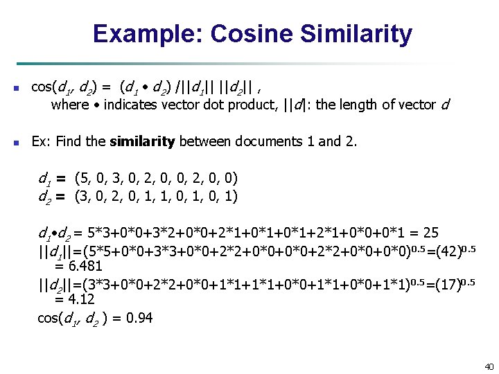
Example: Cosine Similarity n n cos(d 1, d 2) = (d 1 d 2) /||d 1|| ||d 2|| , where indicates vector dot product, ||d|: the length of vector d Ex: Find the similarity between documents 1 and 2. d 1 = (5, 0, 3, 0, 2, 0, 0) d 2 = (3, 0, 2, 0, 1, 1, 0, 1) d 1 d 2 = 5*3+0*0+3*2+0*0+2*1+0*1+2*1+0*0+0*1 = 25 ||d 1||= (5*5+0*0+3*3+0*0+2*2+0*0+0*0) 0. 5=(42)0. 5 = 6. 481 ||d 2||=(3*3+0*0+2*2+0*0+1*1+0*0+1*1) 0. 5=(17)0. 5 = 4. 12 cos(d 1, d 2 ) = 0. 94 40

Summary n Data attribute types: nominal, binary, ordinal, interval-scaled, ratioscaled n Many types of data sets, e. g. , numerical, text, graph, Web, image. n Gain insight into the data by: n Basic statistical data description: central tendency, dispersion, graphical displays n Data visualization: map data onto graphical primitives n Measure data similarity n Above steps are the beginning of data preprocessing. n Many methods have been developed but still an active area of research. 41