Data Mining Classification This lecture node is modified

Data Mining Classification This lecture node is modified based on Lecture Notes for Chapter 4/5 of Introduction to Data Mining by Tan, Steinbach, Kumar, and slides from Jiawei Han for the book of Data Mining – Concepts and Techniqies by Jiawei Han and Micheline Kamber. © Tan, Steinbach, Kumar Introduction to Data Mining 4/18/2004 1

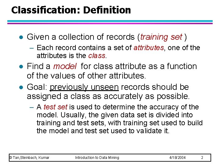
Classification: Definition l Given a collection of records (training set ) – Each record contains a set of attributes, one of the attributes is the class. l l Find a model for class attribute as a function of the values of other attributes. Goal: previously unseen records should be assigned a class as accurately as possible. – A test set is used to determine the accuracy of the model. Usually, the given data set is divided into training and test sets, with training set used to build the model and test set used to validate it. © Tan, Steinbach, Kumar Introduction to Data Mining 4/18/2004 2

Classification Techniques Decision Tree l Naïve Bayes l k. NN Classification l © Tan, Steinbach, Kumar Introduction to Data Mining 4/18/2004 3

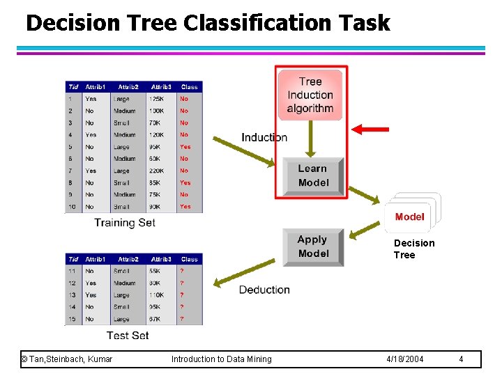
Decision Tree Classification Task Decision Tree © Tan, Steinbach, Kumar Introduction to Data Mining 4/18/2004 4

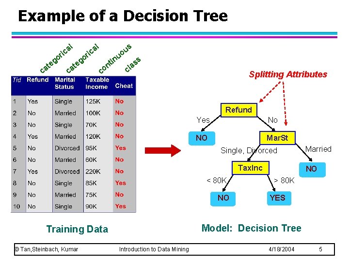
Example of a Decision Tree al ric at c o eg c at al o eg ric in nt co s u o u ss a cl Splitting Attributes Refund Yes No NO Mar. St Single, Divorced Tax. Inc < 80 K NO NO > 80 K YES Model: Decision Tree Training Data © Tan, Steinbach, Kumar Married Introduction to Data Mining 4/18/2004 5

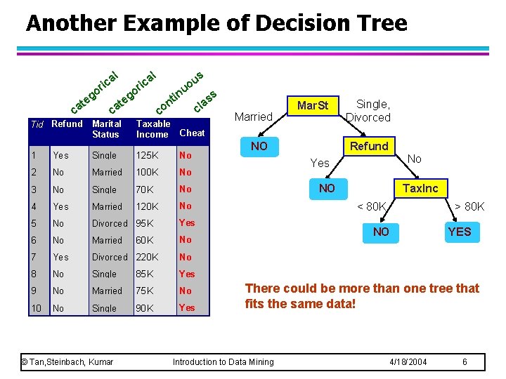
Another Example of Decision Tree l g te ca l a ric o o g te s a ric ca u uo in t n co Tid Refund Marital Status Taxable Income Cheat 1 Yes Single 125 K No 2 No Married 100 K No 3 No Single 70 K No 4 Yes Married 120 K No 5 No Divorced 95 K Yes 6 No Married No 7 Yes Divorced 220 K No 8 No Single 85 K Yes 9 No Married 75 K No 10 No Single 90 K Yes 60 K ss a cl Married Mar. St NO Single, Divorced Refund No Yes NO Tax. Inc < 80 K > 80 K NO YES There could be more than one tree that fits the same data! 10 © Tan, Steinbach, Kumar Introduction to Data Mining 4/18/2004 6

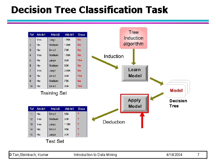
Decision Tree Classification Task Decision Tree © Tan, Steinbach, Kumar Introduction to Data Mining 4/18/2004 7

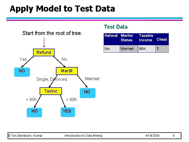
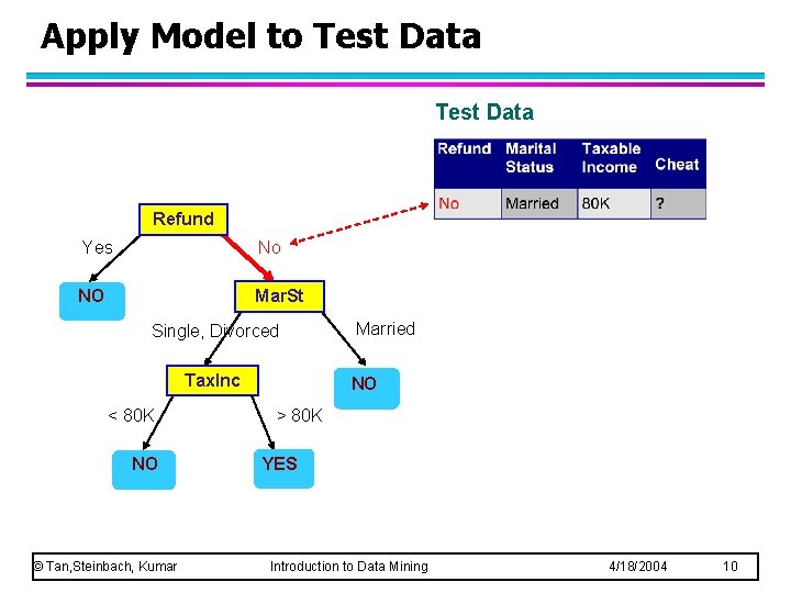
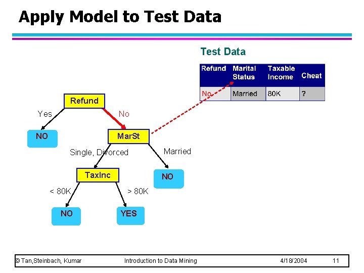
Apply Model to Test Data Start from the root of tree. Refund Yes No NO Mar. St Single, Divorced Tax. Inc < 80 K NO © Tan, Steinbach, Kumar Married NO > 80 K YES Introduction to Data Mining 4/18/2004 8

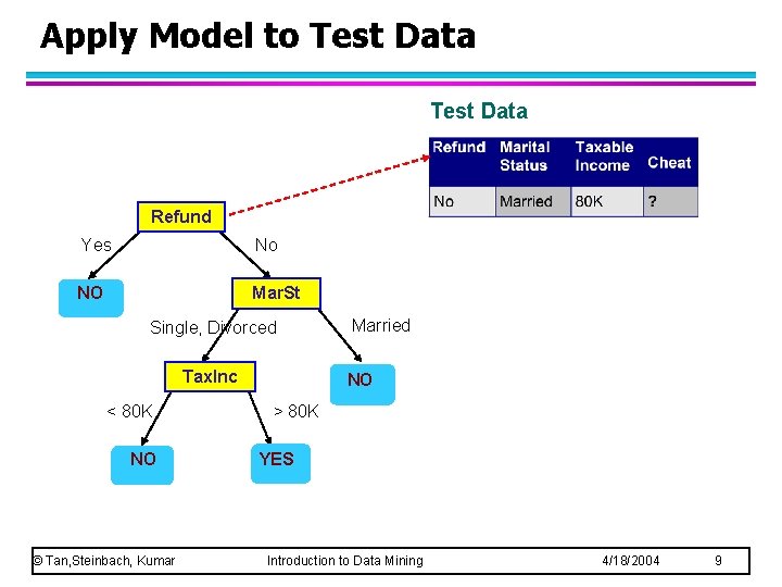
Apply Model to Test Data Refund Yes No NO Mar. St Single, Divorced Tax. Inc < 80 K NO © Tan, Steinbach, Kumar Married NO > 80 K YES Introduction to Data Mining 4/18/2004 9

Apply Model to Test Data Refund Yes No NO Mar. St Single, Divorced Tax. Inc < 80 K NO © Tan, Steinbach, Kumar Married NO > 80 K YES Introduction to Data Mining 4/18/2004 10

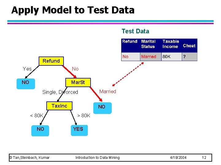
Apply Model to Test Data Refund Yes No NO Mar. St Single, Divorced Tax. Inc < 80 K NO © Tan, Steinbach, Kumar Married NO > 80 K YES Introduction to Data Mining 4/18/2004 11

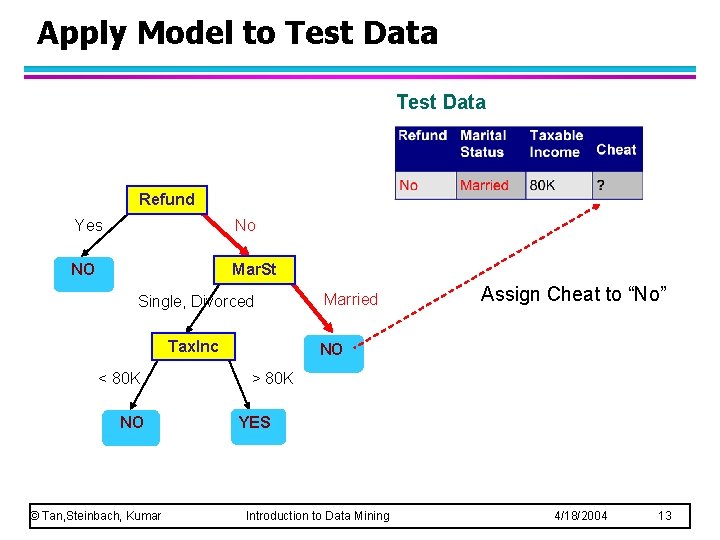
Apply Model to Test Data Refund Yes No NO Mar. St Single, Divorced Tax. Inc < 80 K NO © Tan, Steinbach, Kumar Married NO > 80 K YES Introduction to Data Mining 4/18/2004 12

Apply Model to Test Data Refund Yes No NO Mar. St Single, Divorced Tax. Inc < 80 K NO © Tan, Steinbach, Kumar Married Assign Cheat to “No” NO > 80 K YES Introduction to Data Mining 4/18/2004 13

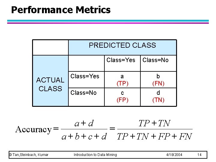
Performance Metrics PREDICTED CLASS Class=Yes ACTUAL CLASS Class=No Class=Yes a (TP) b (FN) Class=No c (FP) d (TN) a+d TP + TN = Accuracy = a + b + c + d TP + TN + FP + FN © Tan, Steinbach, Kumar Introduction to Data Mining 4/18/2004 14

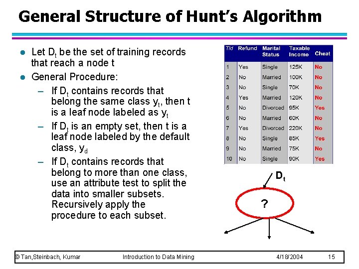
General Structure of Hunt’s Algorithm l l Let Dt be the set of training records that reach a node t General Procedure: – If Dt contains records that belong the same class yt, then t is a leaf node labeled as yt – If Dt is an empty set, then t is a leaf node labeled by the default class, yd – If Dt contains records that belong to more than one class, use an attribute test to split the data into smaller subsets. Recursively apply the procedure to each subset. © Tan, Steinbach, Kumar Introduction to Data Mining Dt ? 4/18/2004 15

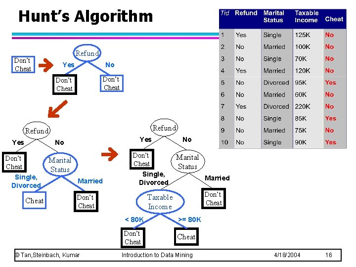
Hunt’s Algorithm Don’t Cheat Refund Yes No Don’t Cheat Single, Divorced Cheat Don’t Cheat Marital Status Married Single, Divorced Marital Status Married Don’t Cheat Taxable Income Don’t Cheat © Tan, Steinbach, Kumar No < 80 K >= 80 K Don’t Cheat Introduction to Data Mining 4/18/2004 16

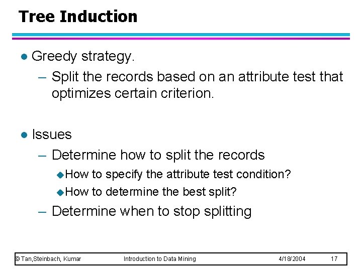
Tree Induction l Greedy strategy. – Split the records based on an attribute test that optimizes certain criterion. l Issues – Determine how to split the records u. How to specify the attribute test condition? u. How to determine the best split? – Determine when to stop splitting © Tan, Steinbach, Kumar Introduction to Data Mining 4/18/2004 17

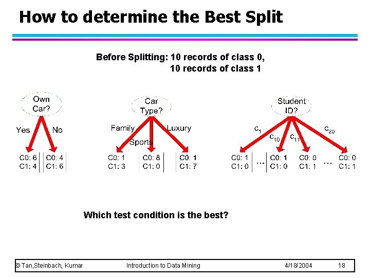
How to determine the Best Split Before Splitting: 10 records of class 0, 10 records of class 1 Which test condition is the best? © Tan, Steinbach, Kumar Introduction to Data Mining 4/18/2004 18

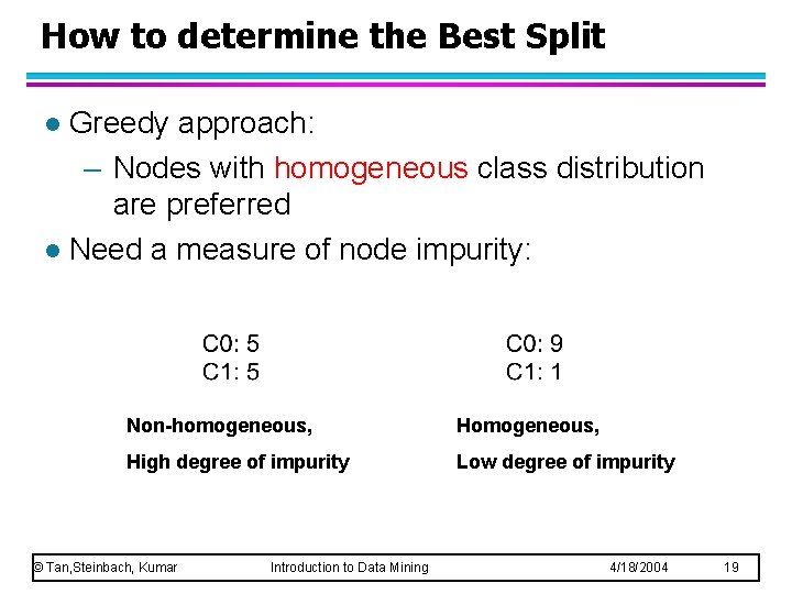
How to determine the Best Split Greedy approach: – Nodes with homogeneous class distribution are preferred l Need a measure of node impurity: l Non-homogeneous, High degree of impurity Low degree of impurity © Tan, Steinbach, Kumar Introduction to Data Mining 4/18/2004 19

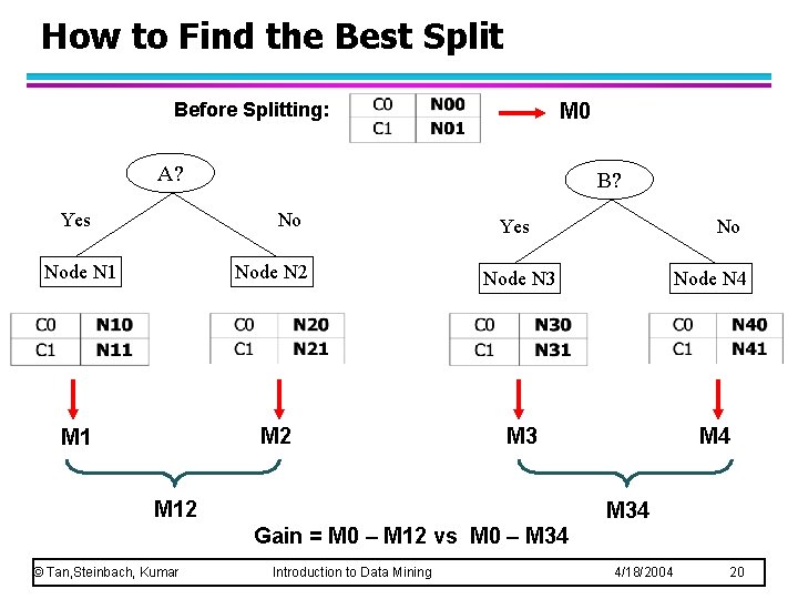
How to Find the Best Split Before Splitting: M 0 A? Yes B? No Yes No Node N 1 Node N 2 Node N 3 Node N 4 M 1 M 2 M 3 M 4 M 12 M 34 Gain = M 0 – M 12 vs M 0 – M 34 © Tan, Steinbach, Kumar Introduction to Data Mining 4/18/2004 20

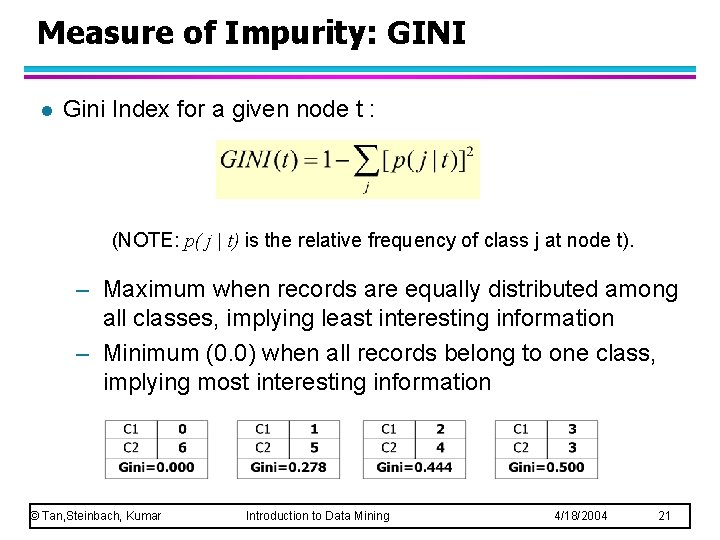
Measure of Impurity: GINI l Gini Index for a given node t : (NOTE: p( j | t) is the relative frequency of class j at node t). – Maximum when records are equally distributed among all classes, implying least interesting information – Minimum (0. 0) when all records belong to one class, implying most interesting information © Tan, Steinbach, Kumar Introduction to Data Mining 4/18/2004 21

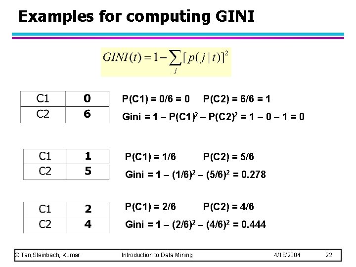
Examples for computing GINI P(C 1) = 0/6 = 0 P(C 2) = 6/6 = 1 Gini = 1 – P(C 1)2 – P(C 2)2 = 1 – 0 – 1 = 0 P(C 1) = 1/6 P(C 2) = 5/6 Gini = 1 – (1/6)2 – (5/6)2 = 0. 278 P(C 1) = 2/6 P(C 2) = 4/6 Gini = 1 – (2/6)2 – (4/6)2 = 0. 444 © Tan, Steinbach, Kumar Introduction to Data Mining 4/18/2004 22

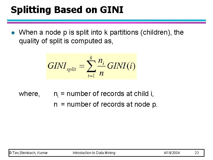
Splitting Based on GINI l When a node p is split into k partitions (children), the quality of split is computed as, where, © Tan, Steinbach, Kumar ni = number of records at child i, n = number of records at node p. Introduction to Data Mining 4/18/2004 23

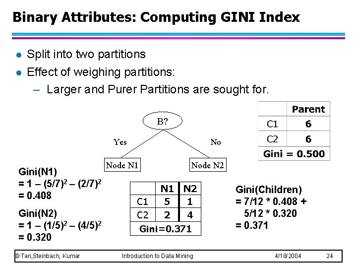
Binary Attributes: Computing GINI Index l l Split into two partitions Effect of weighing partitions: – Larger and Purer Partitions are sought for. B? Yes Gini(N 1) = 1 – (5/7)2 – (2/7)2 = 0. 408 Gini(N 2) = 1 – (1/5)2 – (4/5)2 = 0. 320 © Tan, Steinbach, Kumar No Node N 1 Node N 2 N 1 N 2 C 1 5 1 C 2 2 4 Gini=0. 371 Introduction to Data Mining Gini(Children) = 7/12 * 0. 408 + 5/12 * 0. 320 = 0. 371 4/18/2004 24

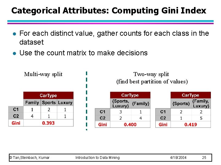
Categorical Attributes: Computing Gini Index l l For each distinct value, gather counts for each class in the dataset Use the count matrix to make decisions Multi-way split © Tan, Steinbach, Kumar Two-way split (find best partition of values) Introduction to Data Mining 4/18/2004 25

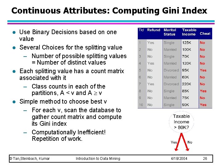
Continuous Attributes: Computing Gini Index l l Use Binary Decisions based on one value Several Choices for the splitting value – Number of possible splitting values = Number of distinct values Each splitting value has a count matrix associated with it – Class counts in each of the partitions, A < v and A v Simple method to choose best v – For each v, scan the database to gather count matrix and compute its Gini index – Computationally Inefficient! Repetition of work. © Tan, Steinbach, Kumar Introduction to Data Mining 4/18/2004 26

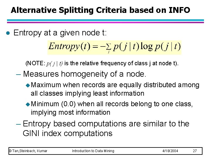
Alternative Splitting Criteria based on INFO l Entropy at a given node t: (NOTE: p( j | t) is the relative frequency of class j at node t). – Measures homogeneity of a node. u Maximum when records are equally distributed among all classes implying least information u Minimum (0. 0) when all records belong to one class, implying most information – Entropy based computations are similar to the GINI index computations © Tan, Steinbach, Kumar Introduction to Data Mining 4/18/2004 27

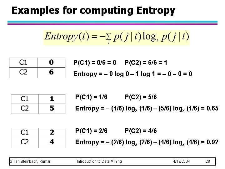
Examples for computing Entropy P(C 1) = 0/6 = 0 P(C 2) = 6/6 = 1 Entropy = – 0 log 0 – 1 log 1 = – 0 = 0 P(C 1) = 1/6 P(C 2) = 5/6 Entropy = – (1/6) log 2 (1/6) – (5/6) log 2 (1/6) = 0. 65 P(C 1) = 2/6 P(C 2) = 4/6 Entropy = – (2/6) log 2 (2/6) – (4/6) log 2 (4/6) = 0. 92 © Tan, Steinbach, Kumar Introduction to Data Mining 4/18/2004 28

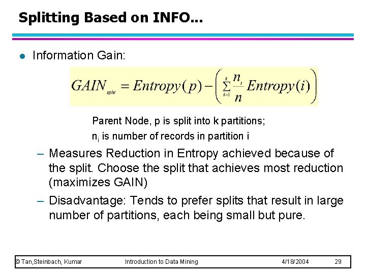
Splitting Based on INFO. . . l Information Gain: Parent Node, p is split into k partitions; ni is number of records in partition i – Measures Reduction in Entropy achieved because of the split. Choose the split that achieves most reduction (maximizes GAIN) – Disadvantage: Tends to prefer splits that result in large number of partitions, each being small but pure. © Tan, Steinbach, Kumar Introduction to Data Mining 4/18/2004 29

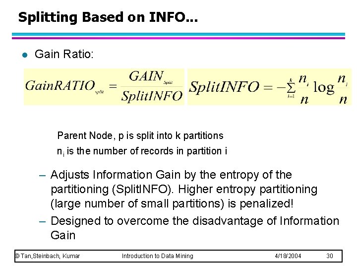
Splitting Based on INFO. . . l Gain Ratio: Parent Node, p is split into k partitions ni is the number of records in partition i – Adjusts Information Gain by the entropy of the partitioning (Split. INFO). Higher entropy partitioning (large number of small partitions) is penalized! – Designed to overcome the disadvantage of Information Gain © Tan, Steinbach, Kumar Introduction to Data Mining 4/18/2004 30

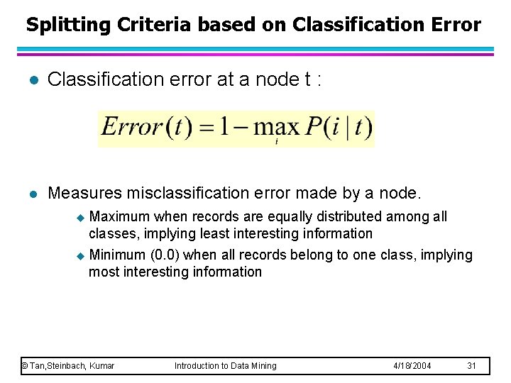
Splitting Criteria based on Classification Error l Classification error at a node t : l Measures misclassification error made by a node. u Maximum when records are equally distributed among all classes, implying least interesting information u Minimum (0. 0) when all records belong to one class, implying most interesting information © Tan, Steinbach, Kumar Introduction to Data Mining 4/18/2004 31

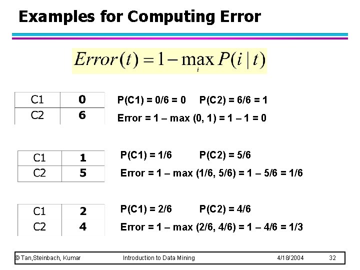
Examples for Computing Error P(C 1) = 0/6 = 0 P(C 2) = 6/6 = 1 Error = 1 – max (0, 1) = 1 – 1 = 0 P(C 1) = 1/6 P(C 2) = 5/6 Error = 1 – max (1/6, 5/6) = 1 – 5/6 = 1/6 P(C 1) = 2/6 P(C 2) = 4/6 Error = 1 – max (2/6, 4/6) = 1 – 4/6 = 1/3 © Tan, Steinbach, Kumar Introduction to Data Mining 4/18/2004 32

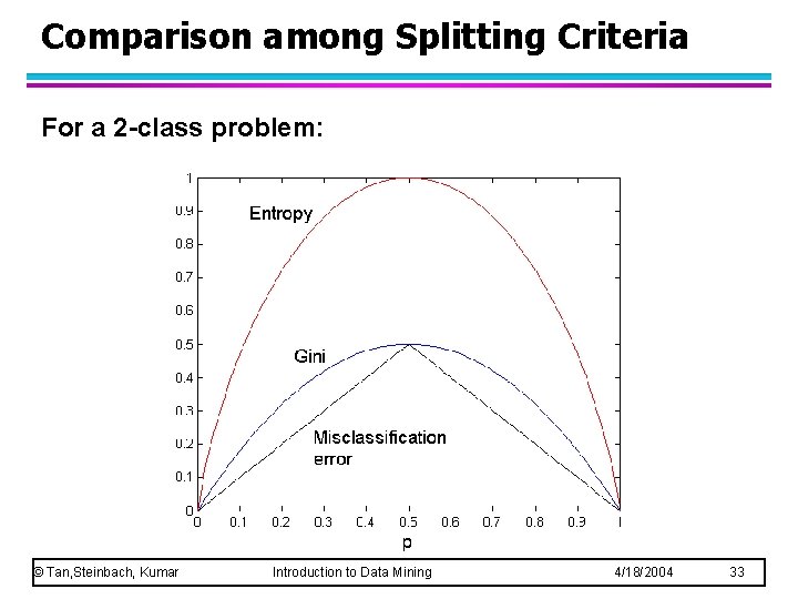
Comparison among Splitting Criteria For a 2 -class problem: © Tan, Steinbach, Kumar Introduction to Data Mining 4/18/2004 33

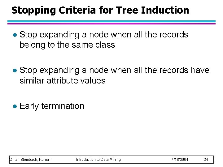
Stopping Criteria for Tree Induction l Stop expanding a node when all the records belong to the same class l Stop expanding a node when all the records have similar attribute values l Early termination © Tan, Steinbach, Kumar Introduction to Data Mining 4/18/2004 34

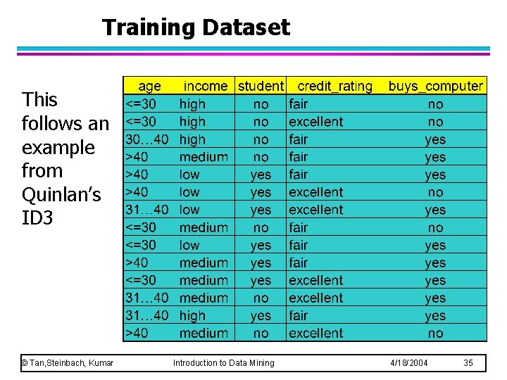
Training Dataset This follows an example from Quinlan’s ID 3 © Tan, Steinbach, Kumar Introduction to Data Mining 4/18/2004 35

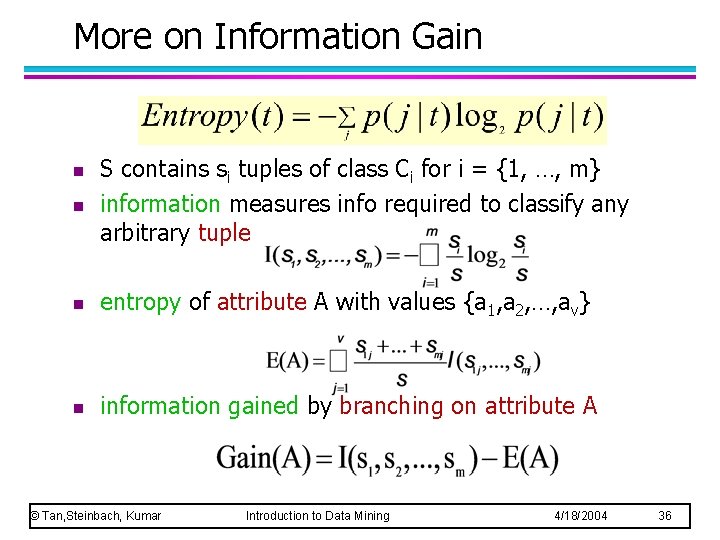
More on Information Gain n S contains si tuples of class Ci for i = {1, …, m} information measures info required to classify any arbitrary tuple n entropy of attribute A with values {a 1, a 2, …, av} n information gained by branching on attribute A n © Tan, Steinbach, Kumar Introduction to Data Mining 4/18/2004 36

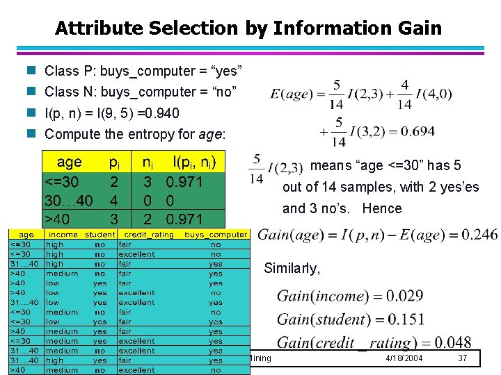
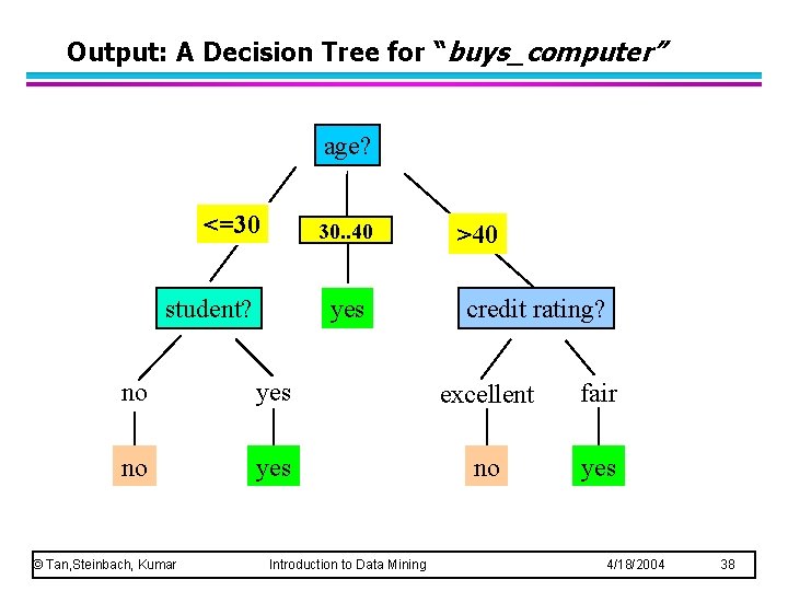
Attribute Selection by Information Gain g Class P: buys_computer = “yes” g Class N: buys_computer = “no” g I(p, n) = I(9, 5) =0. 940 g Compute the entropy for age: means “age <=30” has 5 out of 14 samples, with 2 yes’es and 3 no’s. Hence Similarly, © Tan, Steinbach, Kumar Introduction to Data Mining 4/18/2004 37

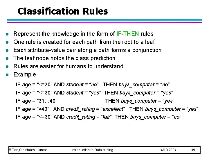
Output: A Decision Tree for “buys_computer” age? <=30 overcast 30. . 40 student? yes >40 credit rating? no yes excellent fair no yes © Tan, Steinbach, Kumar Introduction to Data Mining 4/18/2004 38

Classification Rules l l l Represent the knowledge in the form of IF-THEN rules One rule is created for each path from the root to a leaf Each attribute-value pair along a path forms a conjunction The leaf node holds the class prediction Rules are easier for humans to understand Example IF age = “<=30” AND student = “no” THEN buys_computer = “no” IF age = “<=30” AND student = “yes” THEN buys_computer = “yes” IF age = “ 31… 40” THEN buys_computer = “yes” IF age = “>40” AND credit_rating = “excellent” THEN buys_computer = “yes” IF age = “<=30” AND credit_rating = “fair” THEN buys_computer = “no” © Tan, Steinbach, Kumar Introduction to Data Mining 4/18/2004 39

Decision Tree Based Classification l Advantages: – Inexpensive to construct – Extremely fast at classifying unknown records – Easy to interpret for small-sized trees – Accuracy is comparable to other classification techniques for many simple data sets © Tan, Steinbach, Kumar Introduction to Data Mining 4/18/2004 40

Decision Boundary • Border line between two neighboring regions of different classes is known as decision boundary • Decision boundary is parallel to axes because test condition involves a single attribute at-a-time © Tan, Steinbach, Kumar Introduction to Data Mining 4/18/2004 41

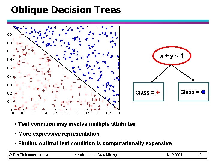
Oblique Decision Trees x+y<1 Class = + Class = • Test condition may involve multiple attributes • More expressive representation • Finding optimal test condition is computationally expensive © Tan, Steinbach, Kumar Introduction to Data Mining 4/18/2004 42

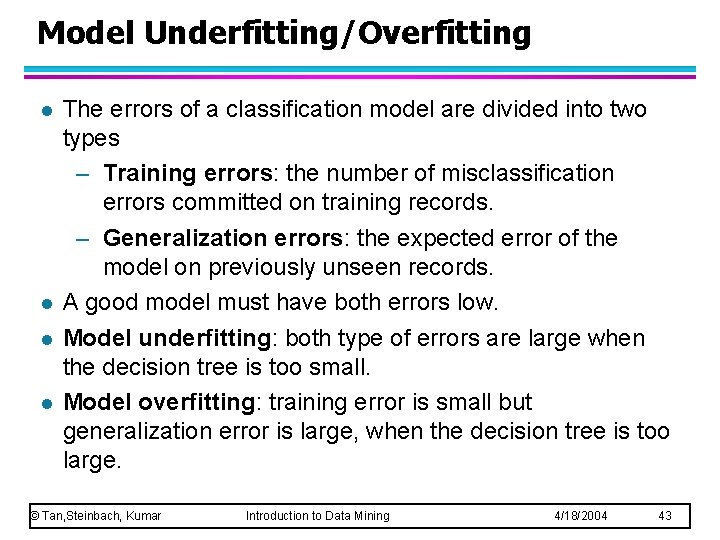
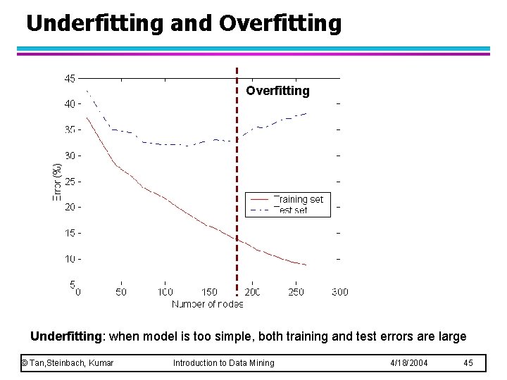
Model Underfitting/Overfitting l l The errors of a classification model are divided into two types – Training errors: the number of misclassification errors committed on training records. – Generalization errors: the expected error of the model on previously unseen records. A good model must have both errors low. Model underfitting: both type of errors are large when the decision tree is too small. Model overfitting: training error is small but generalization error is large, when the decision tree is too large. © Tan, Steinbach, Kumar Introduction to Data Mining 4/18/2004 43

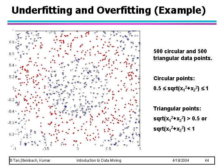
Underfitting and Overfitting (Example) 500 circular and 500 triangular data points. Circular points: 0. 5 sqrt(x 12+x 22) 1 Triangular points: sqrt(x 12+x 22) > 0. 5 or sqrt(x 12+x 22) < 1 © Tan, Steinbach, Kumar Introduction to Data Mining 4/18/2004 44

Underfitting and Overfitting Underfitting: when model is too simple, both training and test errors are large © Tan, Steinbach, Kumar Introduction to Data Mining 4/18/2004 45

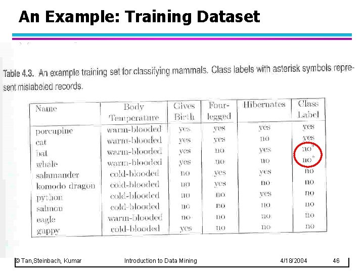
An Example: Training Dataset © Tan, Steinbach, Kumar Introduction to Data Mining 4/18/2004 46

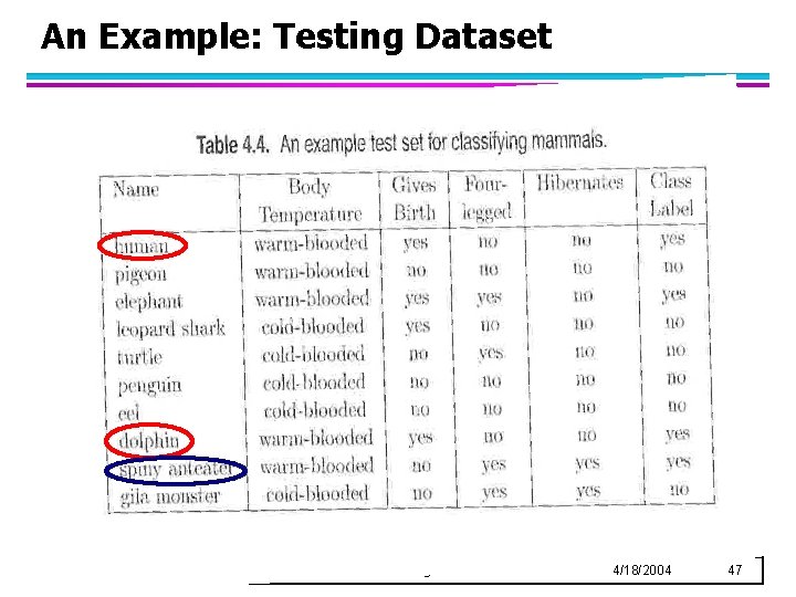
An Example: Testing Dataset © Tan, Steinbach, Kumar Introduction to Data Mining 4/18/2004 47

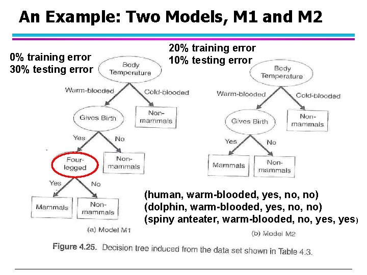
An Example: Two Models, M 1 and M 2 0% training error 30% testing error 20% training error 10% testing error (human, warm-blooded, yes, no) (dolphin, warm-blooded, yes, no) (spiny anteater, warm-blooded, no, yes) © Tan, Steinbach, Kumar Introduction to Data Mining 4/18/2004 48

Occam’s Razor l Given two models of similar generalization errors, one should prefer the simpler model over the more complex model l For complex models, there is a greater chance that it was fitted accidentally by errors in data l Therefore, one should include model complexity when evaluating a model © Tan, Steinbach, Kumar Introduction to Data Mining 4/18/2004 49

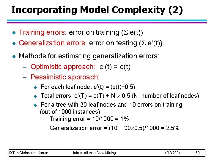
Incorporating Model Complexity (2) l l l Training errors: error on training ( e(t)) Generalization errors: error on testing ( e’(t)) Methods for estimating generalization errors: – Optimistic approach: e’(t) = e(t) – Pessimistic approach: u For each leaf node: e’(t) = (e(t)+0. 5) u Total errors: e’(T) = e(T) + N 0. 5 (N: number of leaf nodes) u For a tree with 30 leaf nodes and 10 errors on training (out of 1000 instances): Training error = 10/1000 = 1% Generalization error = (10 + 30 0. 5)/1000 = 2. 5% © Tan, Steinbach, Kumar Introduction to Data Mining 4/18/2004 50

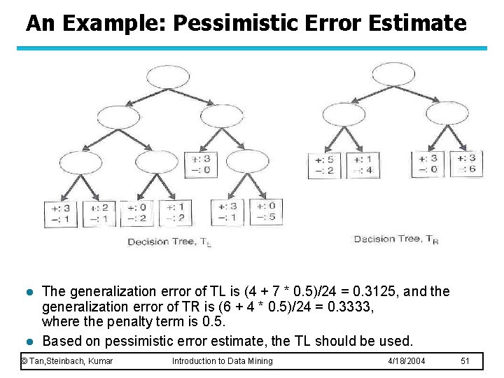
An Example: Pessimistic Error Estimate l l The generalization error of TL is (4 + 7 * 0. 5)/24 = 0. 3125, and the generalization error of TR is (6 + 4 * 0. 5)/24 = 0. 3333, where the penalty term is 0. 5. Based on pessimistic error estimate, the TL should be used. © Tan, Steinbach, Kumar Introduction to Data Mining 4/18/2004 51

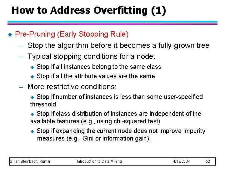
How to Address Overfitting (1) l Pre-Pruning (Early Stopping Rule) – Stop the algorithm before it becomes a fully-grown tree – Typical stopping conditions for a node: u Stop if all instances belong to the same class u Stop if all the attribute values are the same – More restrictive conditions: Stop if number of instances is less than some user-specified threshold u Stop if class distribution of instances are independent of the available features (e. g. , using chi-squared test) u u Stop if expanding the current node does not improve impurity measures (e. g. , Gini or information gain). © Tan, Steinbach, Kumar Introduction to Data Mining 4/18/2004 52

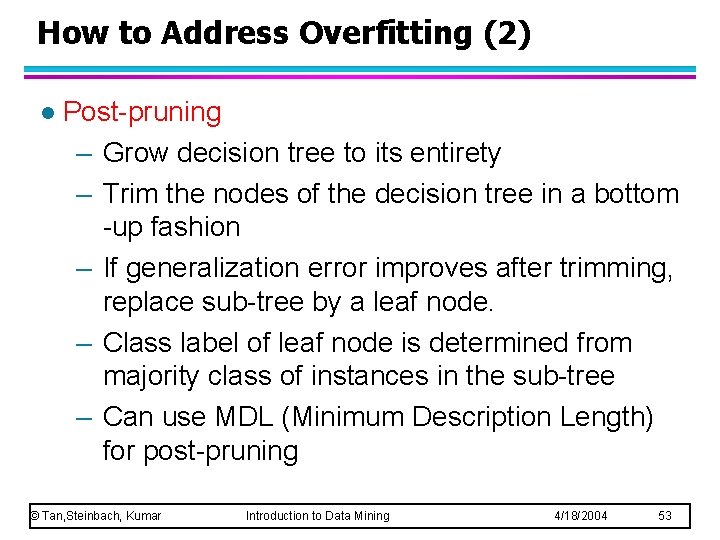
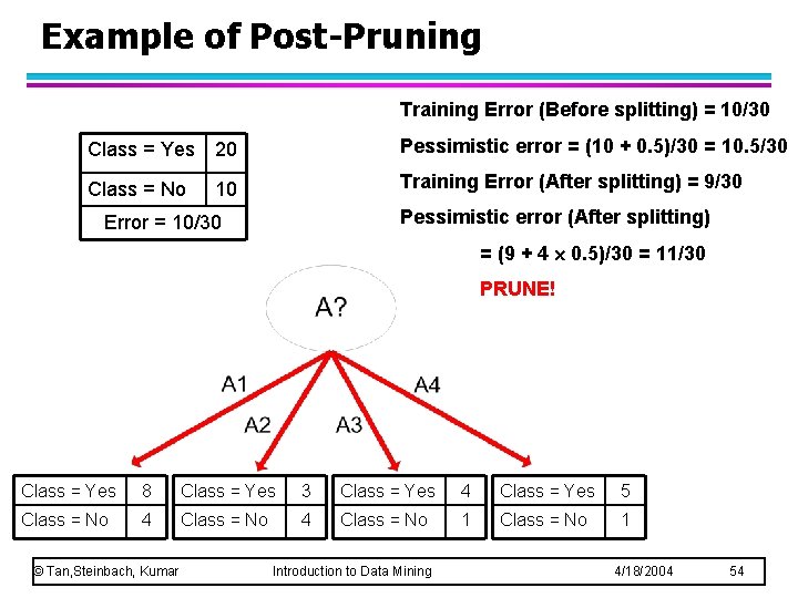
How to Address Overfitting (2) l Post-pruning – Grow decision tree to its entirety – Trim the nodes of the decision tree in a bottom -up fashion – If generalization error improves after trimming, replace sub-tree by a leaf node. – Class label of leaf node is determined from majority class of instances in the sub-tree – Can use MDL (Minimum Description Length) for post-pruning © Tan, Steinbach, Kumar Introduction to Data Mining 4/18/2004 53

Example of Post-Pruning Training Error (Before splitting) = 10/30 Class = Yes 20 Pessimistic error = (10 + 0. 5)/30 = 10. 5/30 Class = No 10 Training Error (After splitting) = 9/30 Pessimistic error (After splitting) Error = 10/30 = (9 + 4 0. 5)/30 = 11/30 PRUNE! Class = Yes 8 Class = Yes 3 Class = Yes 4 Class = Yes 5 Class = No 4 Class = No 1 © Tan, Steinbach, Kumar Introduction to Data Mining 4/18/2004 54