Data Mining Classification contd Recap So far Introduction

Data Mining : Classification (cont’d)

Recap So far: • Introduction to Data Mining • Association Rules • Supervised Classification - Decision tree – using information theory Next • Decision tree using Gini Index (today) • Decision tree summary (today) • Classification using Bayes Method (today) • Unsupervised Classification – Clustering (weeks 6/7) • The term test and Assignment 2 (week 8)

Decision Tree Have considered information theory approach. Used in well known software C 4. 5. Another commonly used approach is called the Gini index. Used in CART and IBM Intelligent Miner. Both approaches are concave measures. The total value of the measure is never less than the total value of the branch nodes. Information gain is always nonnegative. Small entropy or small Gini Index does not guarantee a small classification error.

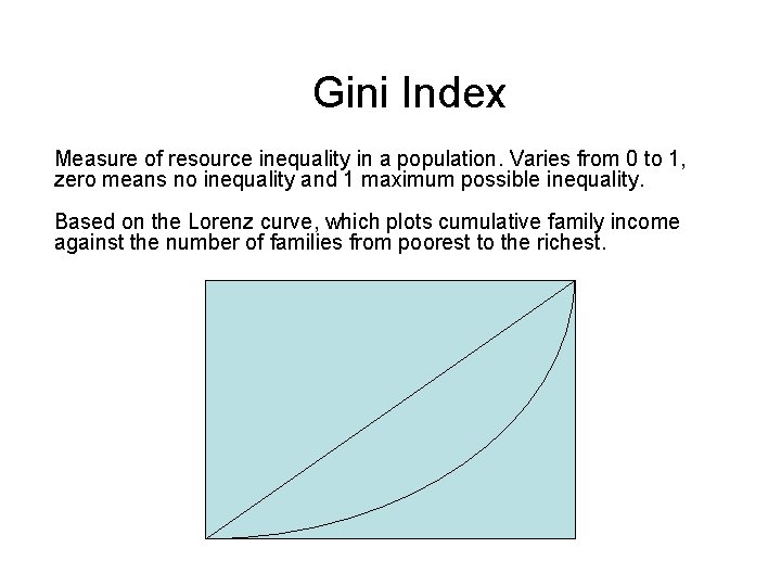
Gini Index Measure of resource inequality in a population. Varies from 0 to 1, zero means no inequality and 1 maximum possible inequality. Based on the Lorenz curve, which plots cumulative family income against the number of families from poorest to the richest.

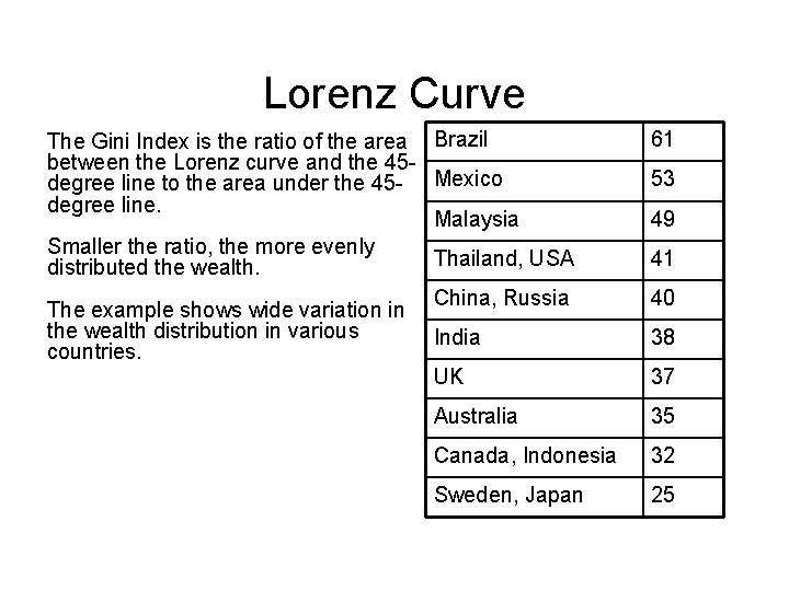
Lorenz Curve The Gini Index is the ratio of the area Brazil between the Lorenz curve and the 45 degree line to the area under the 45 - Mexico degree line. Malaysia Smaller the ratio, the more evenly Thailand, USA distributed the wealth. China, Russia The example shows wide variation in the wealth distribution in various India countries. UK 61 53 49 41 40 38 37 Australia 35 Canada, Indonesia 32 Sweden, Japan 25

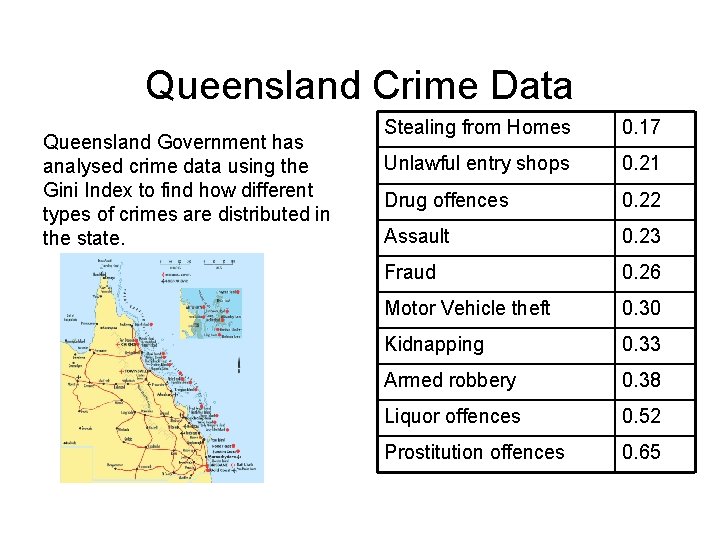
Queensland Crime Data Queensland Government has analysed crime data using the Gini Index to find how different types of crimes are distributed in the state. Stealing from Homes 0. 17 Unlawful entry shops 0. 21 Drug offences 0. 22 Assault 0. 23 Fraud 0. 26 Motor Vehicle theft 0. 30 Kidnapping 0. 33 Armed robbery 0. 38 Liquor offences 0. 52 Prostitution offences 0. 65

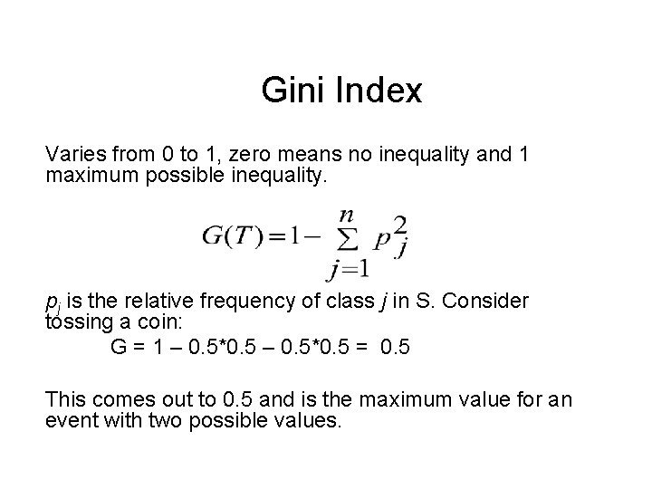
Gini Index Varies from 0 to 1, zero means no inequality and 1 maximum possible inequality. pj is the relative frequency of class j in S. Consider tossing a coin: G = 1 – 0. 5*0. 5 = 0. 5 This comes out to 0. 5 and is the maximum value for an event with two possible values.

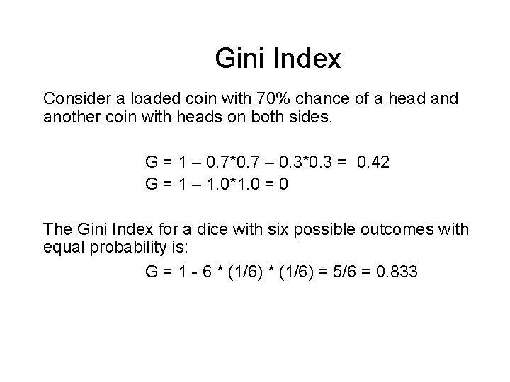
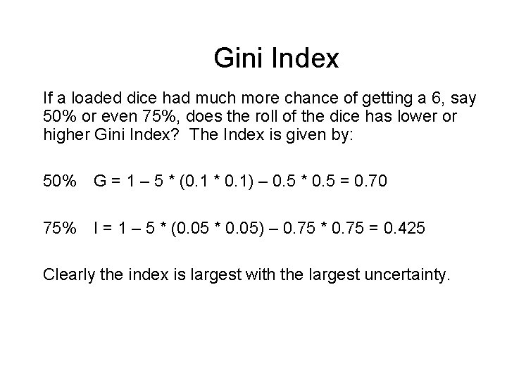
Gini Index Consider a loaded coin with 70% chance of a head another coin with heads on both sides. G = 1 – 0. 7*0. 7 – 0. 3*0. 3 = 0. 42 G = 1 – 1. 0*1. 0 = 0 The Gini Index for a dice with six possible outcomes with equal probability is: G = 1 - 6 * (1/6) = 5/6 = 0. 833

Gini Index If a loaded dice had much more chance of getting a 6, say 50% or even 75%, does the roll of the dice has lower or higher Gini Index? The Index is given by: 50% G = 1 – 5 * (0. 1 * 0. 1) – 0. 5 * 0. 5 = 0. 70 75% I = 1 – 5 * (0. 05 * 0. 05) – 0. 75 * 0. 75 = 0. 425 Clearly the index is largest with the largest uncertainty.

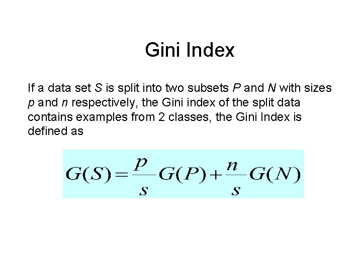
Gini Index If a data set S is split into two subsets P and N with sizes p and n respectively, the Gini index of the split data contains examples from 2 classes, the Gini Index is defined as

Split attribute Once we have computed the Gini Index for all the attributes, how do we select the attribute to split the data? In the case of information theory we selected the attribute with the highest information gain.

Back to the Example

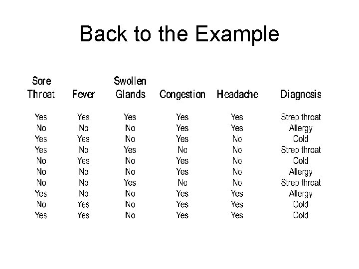
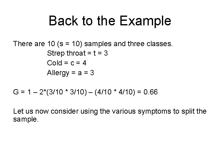
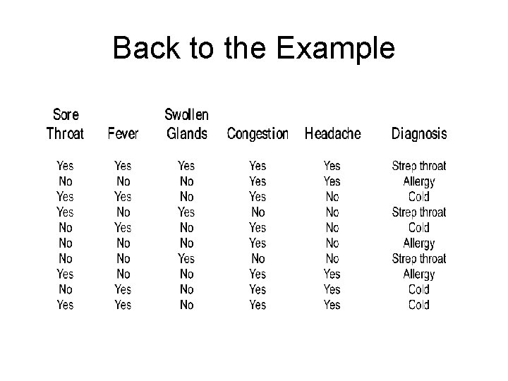
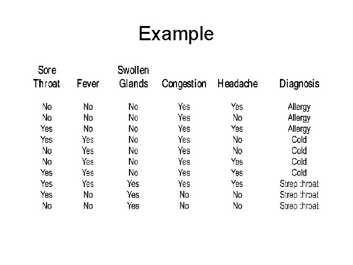
Back to the Example There are 10 (s = 10) samples and three classes. Strep throat = 3 Cold = c = 4 Allergy = a = 3 G = 1 – 2*(3/10 * 3/10) – (4/10 * 4/10) = 0. 66 Let us now consider using the various symptoms to split the sample.

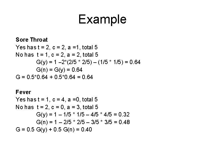
Example Sore Throat Yes has t = 2, c = 2, a =1, total 5 No has t = 1, c = 2, a = 2, total 5 G(y) = 1 – 2*(2/5 * 2/5) – (1/5 * 1/5) = 0. 64 G(n) = G(y) = 0. 64 G = 0. 5*0. 64 + 0. 5*0. 64 = 0. 64 Fever Yes has t = 1, c = 4, a =0, total 5 No has t = 2, c = 0, a = 3, total 5 G(y) = 1 – 1/5 * 1/5 – 4/5 * 4/5 = 0. 32 G(n) = 1 – 2/5 * 2/5 – 3/5 * 3/5 = 0. 48 G = 0. 5 G(y) + 0. 5 G(n) = 0. 40

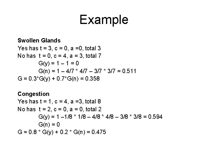
Example Swollen Glands Yes has t = 3, c = 0, a =0, total 3 No has t = 0, c = 4, a = 3, total 7 G(y) = 1 – 1 = 0 G(n) = 1 – 4/7 * 4/7 – 3/7 * 3/7 = 0. 511 G = 0. 3*G(y) + 0. 7*G(n) = 0. 358 Congestion Yes has t = 1, c = 4, a =3, total 8 No has t = 2, c = 0, a = 0, total 2 G(y) = 1 – 1/8 * 1/8 – 4/8 * 4/8 – 3/8 * 3/8 = 0. 594 G(n) = 0 G = 0. 8 * G(y) + 0. 2 * G(n) = 0. 475

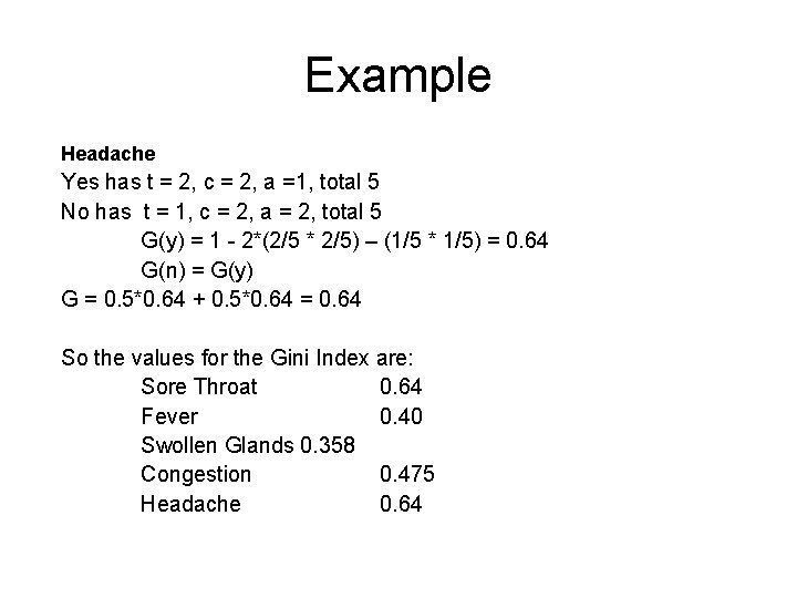
Example Headache Yes has t = 2, c = 2, a =1, total 5 No has t = 1, c = 2, a = 2, total 5 G(y) = 1 - 2*(2/5 * 2/5) – (1/5 * 1/5) = 0. 64 G(n) = G(y) G = 0. 5*0. 64 + 0. 5*0. 64 = 0. 64 So the values for the Gini Index are: Sore Throat 0. 64 Fever 0. 40 Swollen Glands 0. 358 Congestion 0. 475 Headache 0. 64

Example We select the attribute with the smallest value of the index as the split attribute. So the attribute is Swollen Glands. We can now take “Swollen Glands” out of consideration and take three instances where the Swollen Glands symptom value was Yes also out of consideration since they have already been classified. Next we look at the remaining data and remaining attributes and find the next split attribute.

Understanding Decision Trees • Decision trees may be easily represented by rules. • One rule is created for each path from the root to a leaf. • Each internal node is a test and the leaf node gives the class prediction • Example IF swollen glands = yes THEN diagnosis = strep throat IF swollen glands = no and fever = yes then ? ? • Each class may have a number of rules

Overfitting • A decision tree may overfit the training data. A tree overfits the data if an alternative tree has higher accuracy over data other than training data. • Overfit trees tend to have too many branches, some due to outliers • Overfit trees tend to result in poor accuracy for data other than training data • To avoid overfitting it may be desirable to stop some node splits if the split is not really helping classification.

Overfitting Another approach is to build a final tree and then remove branches that do not appear useful. We thus obtain a number of less specific decision trees. Usually data other than training data is required to test such trees obtained by postpruning. Do not have time to get into more details.

Testing • One approach is to divide training data into two parts: one used for building the tree and other for testing the tree. • The data may be randomly divided several times providing several trees and several set of tests. • Statistical tests may be applied if all the data is used for training.

Large Datasets • We have assumed that the datasets are main memory based. What if the data is large and cannot be stored in the main memory? • In some applications the training data may be quite large with many attributes. • New methods have been designed to handle large volumes of data

Decision Tree - Summary • A simple popular method of supervised classification • A decision tree is based on the assumption that there is only one dependent variable i. e. we are trying to predict only one variable. • A decision tree is based on the assumption that all data is categorical. No continuous variable values are used. • Bias – split procedures are often biased towards choosing attributes that have many values.

Bayesian Classification • A different approach: Does not require building of a decision tree. Assume hypothesis that given data belongs to a given class. Calculate probabilities for the hypothesis. This is among the most practical approaches for certain types of problems. • Each training example can incrementally increase/decrease the probability that a hypothesis is correct.

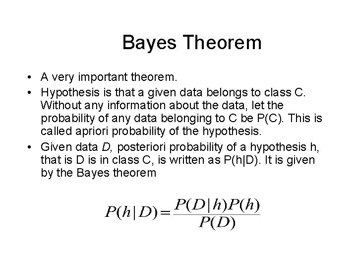
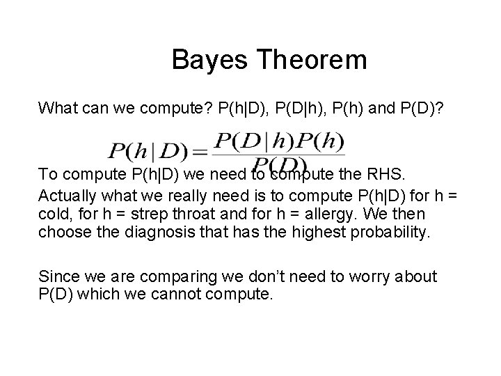
Bayes Theorem • A very important theorem. • Hypothesis is that a given data belongs to class C. Without any information about the data, let the probability of any data belonging to C be P(C). This is called apriori probability of the hypothesis. • Given data D, posteriori probability of a hypothesis h, that is D is in class C, is written as P(h|D). It is given by the Bayes theorem

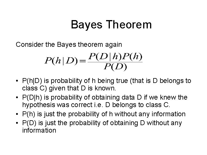
Bayes Theorem Consider the Bayes theorem again • P(h|D) is probability of h being true (that is D belongs to class C) given that D is known. • P(D|h) is probability of obtaining data D if we knew the hypothesis was correct i. e. D belongs to class C. • P(h) is just the probability of h without any information • P(D) is just the probability of obtaining D without any information

Back to the Example

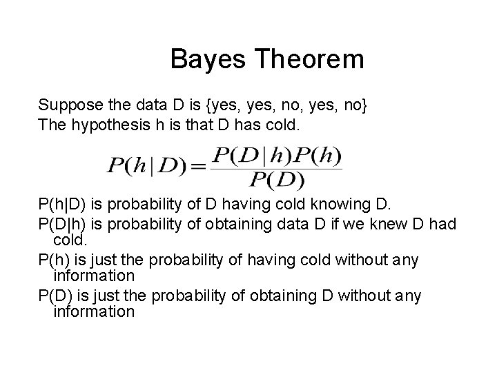
Bayes Theorem Suppose the data D is {yes, no, yes, no} The hypothesis h is that D has cold. P(h|D) is probability of D having cold knowing D. P(D|h) is probability of obtaining data D if we knew D had cold. P(h) is just the probability of having cold without any information P(D) is just the probability of obtaining D without any information

Bayes Theorem What can we compute? P(h|D), P(D|h), P(h) and P(D)? To compute P(h|D) we need to compute the RHS. Actually what we really need is to compute P(h|D) for h = cold, for h = strep throat and for h = allergy. We then choose the diagnosis that has the highest probability. Since we are comparing we don’t need to worry about P(D) which we cannot compute.

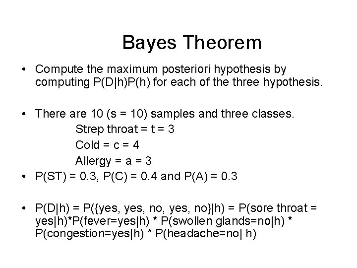
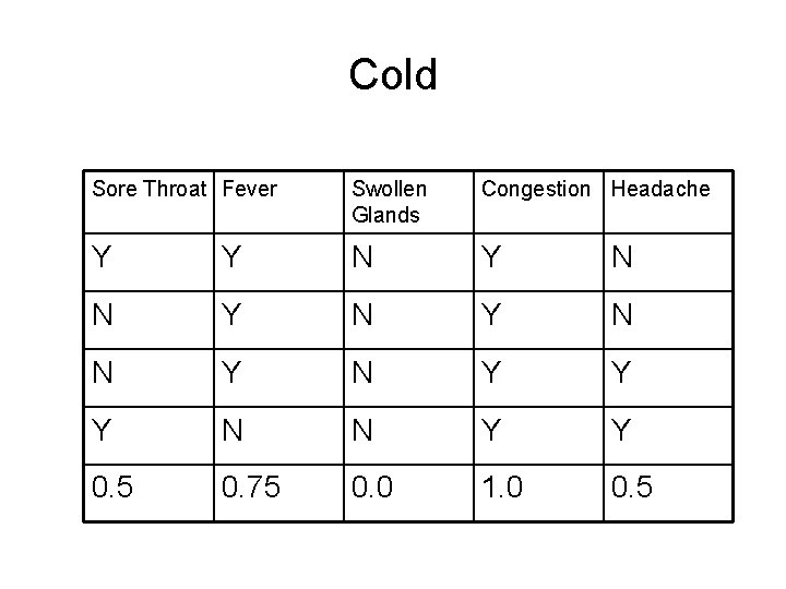
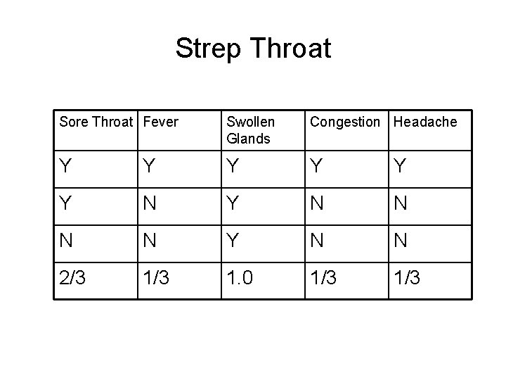
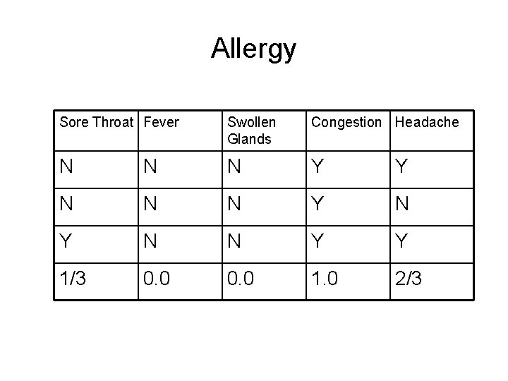
Bayes Theorem • Compute the maximum posteriori hypothesis by computing P(D|h)P(h) for each of the three hypothesis. • There are 10 (s = 10) samples and three classes. Strep throat = 3 Cold = c = 4 Allergy = a = 3 • P(ST) = 0. 3, P(C) = 0. 4 and P(A) = 0. 3 • P(D|h) = P({yes, no, yes, no}|h) = P(sore throat = yes|h)*P(fever=yes|h) * P(swollen glands=no|h) * P(congestion=yes|h) * P(headache=no| h)

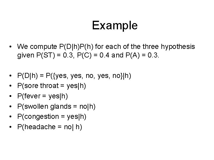
Example • We compute P(D|h)P(h) for each of the three hypothesis given P(ST) = 0. 3, P(C) = 0. 4 and P(A) = 0. 3. • • • P(D|h) = P({yes, no, yes, no}|h) P(sore throat = yes|h) P(fever = yes|h) P(swollen glands = no|h) P(congestion = yes|h) P(headache = no| h)

Example

Cold Sore Throat Fever Swollen Glands Congestion Headache Y Y N Y N Y Y Y N N Y Y 0. 5 0. 75 0. 0 1. 0 0. 5

Strep Throat Sore Throat Fever Swollen Glands Congestion Headache Y Y Y N Y N N 2/3 1. 0 1/3

Allergy Sore Throat Fever Swollen Glands Congestion Headache N N N Y Y N N N Y Y 1/3 0. 0 1. 0 2/3

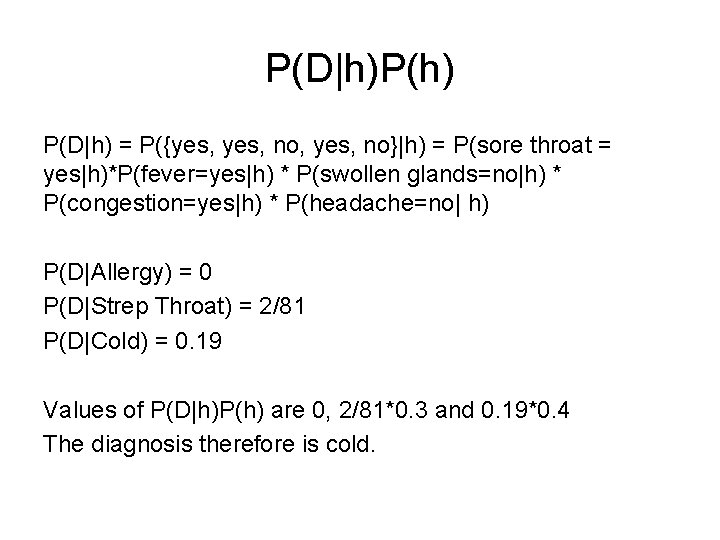
P(D|h)P(h) P(D|h) = P({yes, no, yes, no}|h) = P(sore throat = yes|h)*P(fever=yes|h) * P(swollen glands=no|h) * P(congestion=yes|h) * P(headache=no| h) P(D|Allergy) = 0 P(D|Strep Throat) = 2/81 P(D|Cold) = 0. 19 Values of P(D|h)P(h) are 0, 2/81*0. 3 and 0. 19*0. 4 The diagnosis therefore is cold.

Assumptions • Assuming that attributes are independent • Assuming that the training sample is a good sample to estimate probabilities. • These assumptions are often not true in practice, as attributes are often correlated. • Other techniques have been designed to overcome this limitation.

Summary • Supervised classification • Decision tree using information measure and Gini Index • Pruning and Testing • Bayes Theorem