Data Mining Classification Basic Concepts Decision Trees and
Data Mining Classification: Basic Concepts, Decision Trees, and Model Evaluation Lecture Notes for Chapter 4 Part III Introduction to Data Mining by Tan, Steinbach, Kumar Adapted by Qiang Yang (2010) © Tan, Steinbach, Kumar Introduction to Data Mining 4/18/2004 1
Practical Issues of Classification l Underfitting and Overfitting l Missing Values l Costs of Classification © Tan, Steinbach, Kumar Introduction to Data Mining 4/18/2004 2
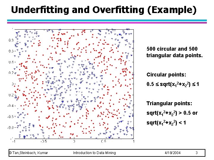
Underfitting and Overfitting (Example) 500 circular and 500 triangular data points. Circular points: 0. 5 sqrt(x 12+x 22) 1 Triangular points: sqrt(x 12+x 22) > 0. 5 or sqrt(x 12+x 22) < 1 © Tan, Steinbach, Kumar Introduction to Data Mining 4/18/2004 3
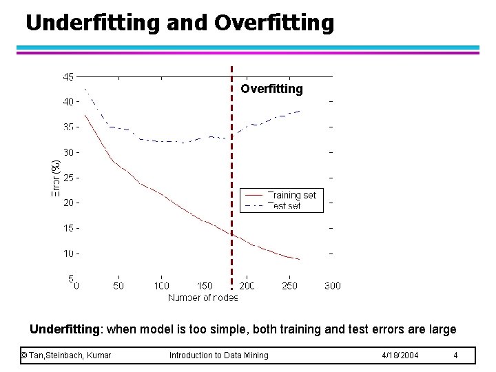
Underfitting and Overfitting Underfitting: when model is too simple, both training and test errors are large © Tan, Steinbach, Kumar Introduction to Data Mining 4/18/2004 4
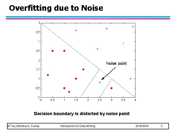
Overfitting due to Noise Decision boundary is distorted by noise point © Tan, Steinbach, Kumar Introduction to Data Mining 4/18/2004 5
Notes on Overfitting l Overfitting results in decision trees that are more complex than necessary l Training error no longer provides a good estimate of how well the tree will perform on previously unseen records l Need new ways for estimating errors © Tan, Steinbach, Kumar Introduction to Data Mining 4/18/2004 6
Estimating Generalization Errors l l l Re-substitution errors: error on training ( e(t) ) Generalization errors: error on testing ( e’(t)) Methods for estimating generalization errors: – Optimistic approach: e’(t) = e(t) – Pessimistic approach: For each leaf node: e’(t) = (e(t)+0. 5) u Total error counts: e’(T) = e(T) + N 0. 5 (N: number of leaf nodes) u For a tree with 30 leaf nodes and 10 errors on training (out of 1000 instances): Training error = 10/1000 = 1% Generalization error = (10 + 30 0. 5)/1000 = 2. 5% u – Reduced error pruning (REP): u uses validation data set to estimate generalization error © Tan, Steinbach, Kumar Introduction to Data Mining 4/18/2004 7
Occam’s Razor l Given two models of similar generalization errors, one should prefer the simpler model over the more complex model – For complex models, there is a greater chance that it was fitted accidentally by errors in data – Therefore, one should include model complexity when evaluating a model © Tan, Steinbach, Kumar Introduction to Data Mining 4/18/2004 8
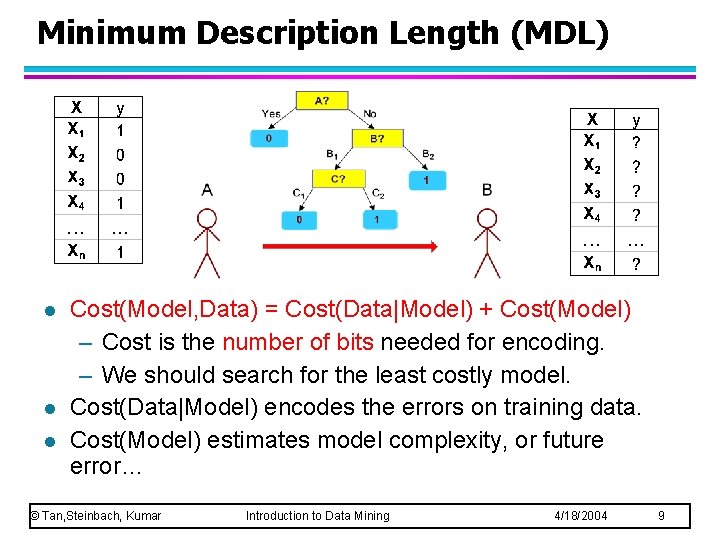
Minimum Description Length (MDL) l l l Cost(Model, Data) = Cost(Data|Model) + Cost(Model) – Cost is the number of bits needed for encoding. – We should search for the least costly model. Cost(Data|Model) encodes the errors on training data. Cost(Model) estimates model complexity, or future error… © Tan, Steinbach, Kumar Introduction to Data Mining 4/18/2004 9
How to Address Overfitting in Decision Trees l Pre-Pruning (Early Stopping Rule) – Stop the algorithm before it becomes a fully-grown tree – Typical stopping conditions for a node: u Stop if all instances belong to the same class u Stop if all the attribute values are the same – More restrictive conditions: Stop if number of instances is less than some user-specified threshold u Stop if class distribution of instances are independent of the available features (e. g. , using 2 test) u u Stop if expanding the current node does not improve impurity measures (e. g. , Gini or information gain). © Tan, Steinbach, Kumar Introduction to Data Mining 4/18/2004 10
How to Address Overfitting… l Post-pruning – Grow decision tree to its entirety – Trim the nodes of the decision tree in a bottom-up fashion – If generalization error improves after trimming, replace sub-tree by a leaf node. u. Heuristic: Class label of leaf node is determined from majority class of instances in the sub-tree generalization error count = error count + 0. 5*N, where N is the number of leaf nodes, u u. This is a heuristic used in some algorithms, but there are other ways using statistics © Tan, Steinbach, Kumar Introduction to Data Mining 4/18/2004 11
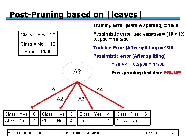
Post-Pruning based on |leaves| Training Error (Before splitting) = 10/30 Class = Yes 20 Class = No 10 Pessimistic error (Before splitting) = (10 + 1 X 0. 5)/30 = 10. 5/30 Training Error (After splitting) = 9/30 Error = 10/30 Pessimistic error (After splitting) = (9 + 4 0. 5)/30 = 11/30 Post-pruning decision: PRUNE! Class = Yes 8 Class = Yes 3 Class = Yes 4 Class = Yes 5 Class = No 4 Class = No 1 © Tan, Steinbach, Kumar Introduction to Data Mining 4/18/2004 12
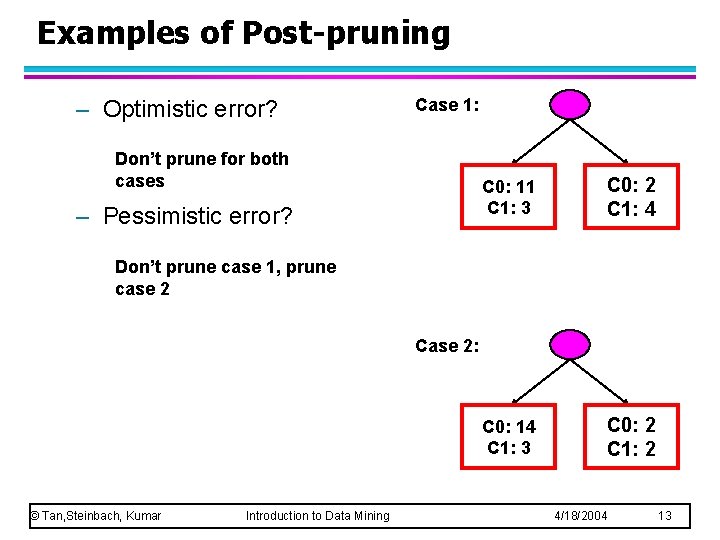
Examples of Post-pruning – Optimistic error? Case 1: Don’t prune for both cases – Pessimistic error? C 0: 11 C 1: 3 C 0: 2 C 1: 4 C 0: 14 C 1: 3 C 0: 2 C 1: 2 Don’t prune case 1, prune case 2 Case 2: © Tan, Steinbach, Kumar Introduction to Data Mining 4/18/2004 13
Data Fragmentation l Number of instances gets smaller as you traverse down the tree Number of instances at the leaf nodes could be too small to make any statistically significant decision l Solution: limit number of instances per leaf node >= a user given value n. l © Tan, Steinbach, Kumar Introduction to Data Mining 4/18/2004 14
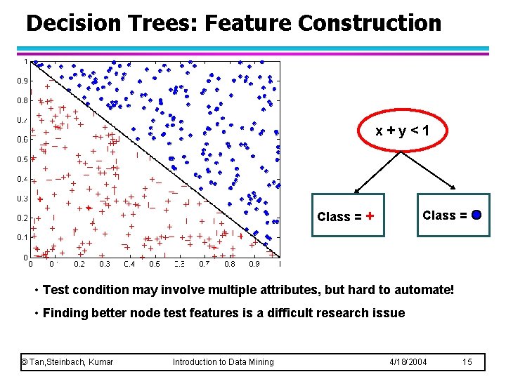
Decision Trees: Feature Construction x+y<1 Class = + Class = • Test condition may involve multiple attributes, but hard to automate! • Finding better node test features is a difficult research issue © Tan, Steinbach, Kumar Introduction to Data Mining 4/18/2004 15
Model Evaluation l Metrics for Performance Evaluation – How to evaluate the performance of a model? l Methods for Performance Evaluation – How to obtain reliable estimates? l Methods for Model Comparison – How to compare the relative performance among competing models? © Tan, Steinbach, Kumar Introduction to Data Mining 4/18/2004 16
Model Evaluation l Metrics for Performance Evaluation – How to evaluate the performance of a model? l Methods for Performance Evaluation – How to obtain reliable estimates? l Methods for Model Comparison – How to compare the relative performance among competing models? © Tan, Steinbach, Kumar Introduction to Data Mining 4/18/2004 17
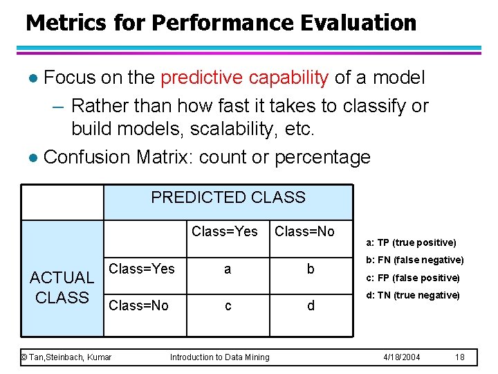
Metrics for Performance Evaluation Focus on the predictive capability of a model – Rather than how fast it takes to classify or build models, scalability, etc. l Confusion Matrix: count or percentage l PREDICTED CLASS Class=Yes ACTUAL CLASS Class=No © Tan, Steinbach, Kumar a c Introduction to Data Mining Class=No b d a: TP (true positive) b: FN (false negative) c: FP (false positive) d: TN (true negative) 4/18/2004 18
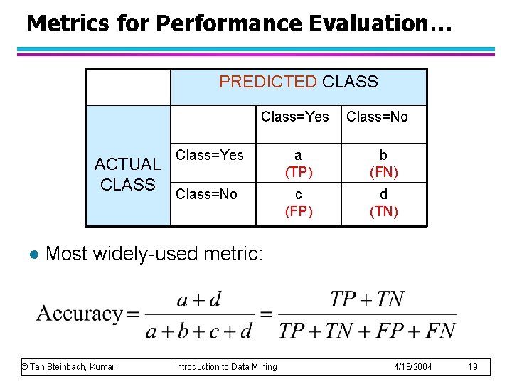
Metrics for Performance Evaluation… PREDICTED CLASS Class=Yes ACTUAL CLASS l Class=No Class=Yes a (TP) b (FN) Class=No c (FP) d (TN) Most widely-used metric: © Tan, Steinbach, Kumar Introduction to Data Mining 4/18/2004 19
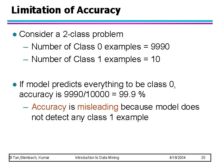
Limitation of Accuracy l Consider a 2 -class problem – Number of Class 0 examples = 9990 – Number of Class 1 examples = 10 l If model predicts everything to be class 0, accuracy is 9990/10000 = 99. 9 % – Accuracy is misleading because model does not detect any class 1 example © Tan, Steinbach, Kumar Introduction to Data Mining 4/18/2004 20
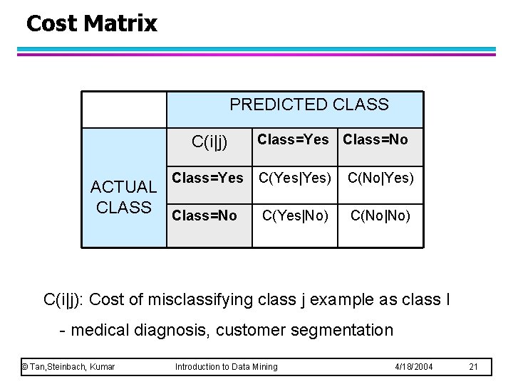
Cost Matrix PREDICTED CLASS C(i|j) Class=Yes ACTUAL CLASS Class=No Class=Yes Class=No C(Yes|Yes) C(No|Yes) C(Yes|No) C(No|No) C(i|j): Cost of misclassifying class j example as class I - medical diagnosis, customer segmentation © Tan, Steinbach, Kumar Introduction to Data Mining 4/18/2004 21
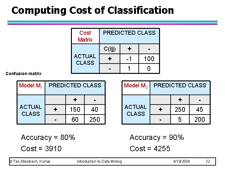
Computing Cost of Classification Cost Matrix PREDICTED CLASS ACTUAL CLASS Confusion matrix Model M 1 C(i|j) + -1 100 - 1 0 PREDICTED CLASS ACTUAL CLASS + - + 150 40 - 60 250 Accuracy = 80% Cost = 3910 © Tan, Steinbach, Kumar Model M 2 ACTUAL CLASS PREDICTED CLASS + - + 250 45 - 5 200 Accuracy = 90% Cost = 4255 Introduction to Data Mining 4/18/2004 22
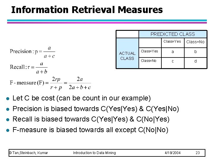
Information Retrieval Measures PREDICTED CLASS ACTUAL CLASS l l Class=Yes Class=No Class=Yes a b Class=No c d Let C be cost (can be count in our example) Precision is biased towards C(Yes|Yes) & C(Yes|No) Recall is biased towards C(Yes|Yes) & C(No|Yes) F-measure is biased towards all except C(No|No) © Tan, Steinbach, Kumar Introduction to Data Mining 4/18/2004 23
Model Evaluation l Metrics for Performance Evaluation – How to evaluate the performance of a model? l Methods for Performance Evaluation – How to obtain reliable estimates? l Methods for Model Comparison – How to compare the relative performance among competing models? © Tan, Steinbach, Kumar Introduction to Data Mining 4/18/2004 24
Methods of Estimation Holdout – Reserve 2/3 for training and 1/3 for testing l Cross validation – Partition data into k disjoint subsets – k-fold: train on k-1 partitions, test on the remaining one – Leave-one-out: k=n l © Tan, Steinbach, Kumar Introduction to Data Mining 4/18/2004 25
Test of Significance (Sections 4. 5, 4. 6 of TSK Book) l Given two models: – Model M 1: accuracy = 85%, tested on 30 instances – Model M 2: accuracy = 75%, tested on 5000 instances l Can we say M 1 is better than M 2? – How much confidence can we place on accuracy of M 1 and M 2? – Can the difference in performance measure be explained as a result of random fluctuations in the test set? © Tan, Steinbach, Kumar Introduction to Data Mining 4/18/2004 26
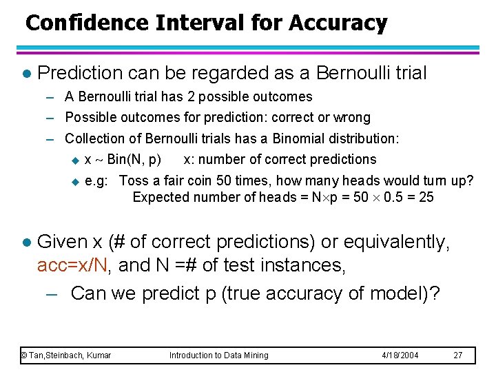
Confidence Interval for Accuracy l Prediction can be regarded as a Bernoulli trial – A Bernoulli trial has 2 possible outcomes – Possible outcomes for prediction: correct or wrong – Collection of Bernoulli trials has a Binomial distribution: u x Bin(N, p) x: number of correct predictions u e. g: Toss a fair coin 50 times, how many heads would turn up? Expected number of heads = N p = 50 0. 5 = 25 l Given x (# of correct predictions) or equivalently, acc=x/N, and N =# of test instances, – Can we predict p (true accuracy of model)? © Tan, Steinbach, Kumar Introduction to Data Mining 4/18/2004 27
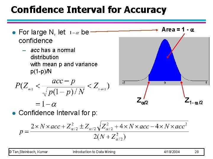
Confidence Interval for Accuracy l For large N, let confidence Area = 1 - be – acc has a normal distribution with mean p and variance p(1 -p)/N Z /2 l Z 1 - /2 Confidence Interval for p: © Tan, Steinbach, Kumar Introduction to Data Mining 4/18/2004 28
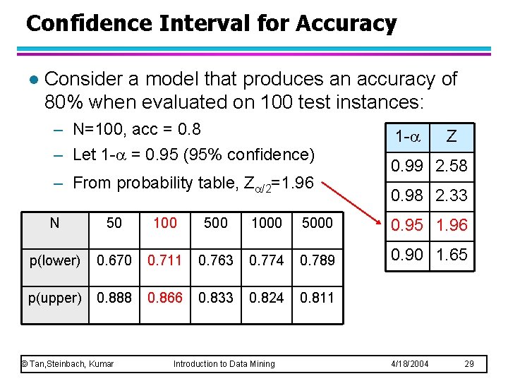
Confidence Interval for Accuracy l Consider a model that produces an accuracy of 80% when evaluated on 100 test instances: – N=100, acc = 0. 8 – Let 1 - = 0. 95 (95% confidence) – From probability table, Z /2=1. 96 1 - Z 0. 99 2. 58 0. 98 2. 33 N 50 100 500 1000 5000 0. 95 1. 96 p(lower) 0. 670 0. 711 0. 763 0. 774 0. 789 0. 90 1. 65 p(upper) 0. 888 0. 866 0. 833 0. 824 0. 811 © Tan, Steinbach, Kumar Introduction to Data Mining 4/18/2004 29
ROC (Receiver Operating Characteristic) l l l l Page 298 of TSK book. Many applications care about ranking (give a queue from the most likely to the least likely) Examples… Which ranking order is better? ROC: Developed in 1950 s for signal detection theory to analyze noisy signals – Characterize the trade-off between positive hits and false alarms ROC curve plots TP (on the y-axis) against FP (on the x-axis) Performance of each classifier represented as a point on the ROC curve – changing the threshold of algorithm, sample distribution or cost matrix changes the location of the point © Tan, Steinbach, Kumar Introduction to Data Mining 4/18/2004 30
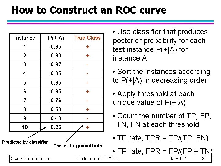
How to Construct an ROC curve Instance P(+|A) True Class 1 0. 95 + 2 0. 93 + 3 0. 87 - 4 0. 85 - 5 0. 85 - 6 0. 85 + 7 0. 76 - 8 0. 53 + 9 0. 43 - 10 0. 25 + Predicted by classifier © Tan, Steinbach, Kumar • Use classifier that produces posterior probability for each test instance P(+|A) for instance A • Sort the instances according to P(+|A) in decreasing order • Apply threshold at each unique value of P(+|A) • Count the number of TP, FP, TN, FN at each threshold • TP rate, TPR = TP/(TP+FN) This is the ground truth • FP rate, FPR = FP/(FP + TN) Introduction to Data Mining 4/18/2004 31
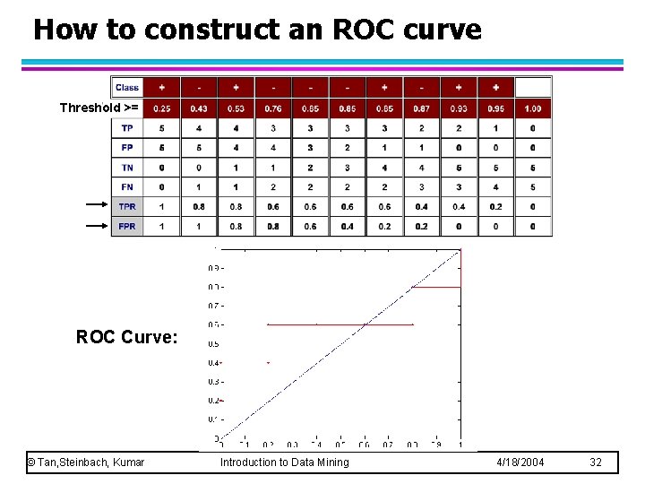
How to construct an ROC curve Threshold >= ROC Curve: © Tan, Steinbach, Kumar Introduction to Data Mining 4/18/2004 32
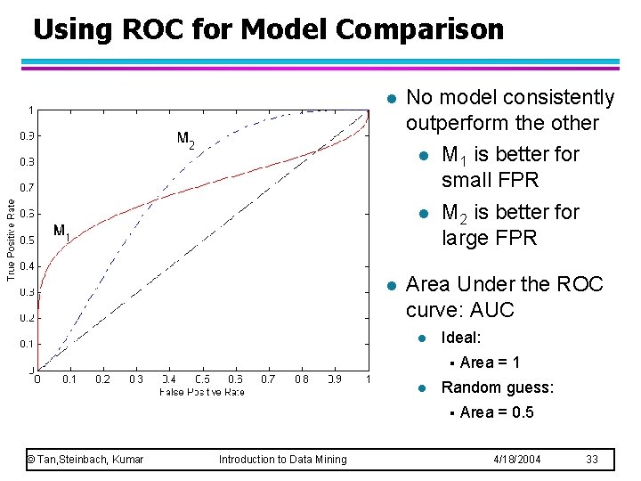
Using ROC for Model Comparison l No model consistently outperform the other l M 1 is better for small FPR l M 2 is better for large FPR l Area Under the ROC curve: AUC l Ideal: § l Random guess: § © Tan, Steinbach, Kumar Introduction to Data Mining Area = 1 Area = 0. 5 4/18/2004 33
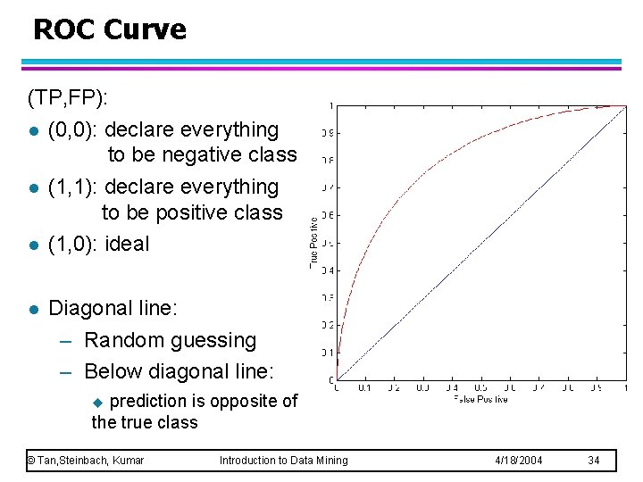
ROC Curve (TP, FP): l (0, 0): declare everything to be negative class l (1, 1): declare everything to be positive class l (1, 0): ideal l Diagonal line: – Random guessing – Below diagonal line: prediction is opposite of the true class u © Tan, Steinbach, Kumar Introduction to Data Mining 4/18/2004 34
- Slides: 34