Data Mining Classification Alternative Techniques Lecture Notes for
- Slides: 59

Data Mining Classification: Alternative Techniques Lecture Notes for Chapter 5 Introduction to Data Mining by Tan, Steinbach, Kumar © Tan, Steinbach, Kumar Introduction to Data Mining 4/18/2004 1

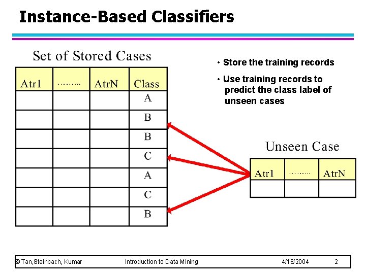
Instance-Based Classifiers • Store the training records • Use training records to predict the class label of unseen cases © Tan, Steinbach, Kumar Introduction to Data Mining 4/18/2004 2

Instance Based Classifiers l Examples: – Rote-learner Memorizes entire training data and performs classification only if attributes of record match one of the training examples exactly u – Nearest neighbor Uses k “closest” points (nearest neighbors) for performing classification u © Tan, Steinbach, Kumar Introduction to Data Mining 4/18/2004 3

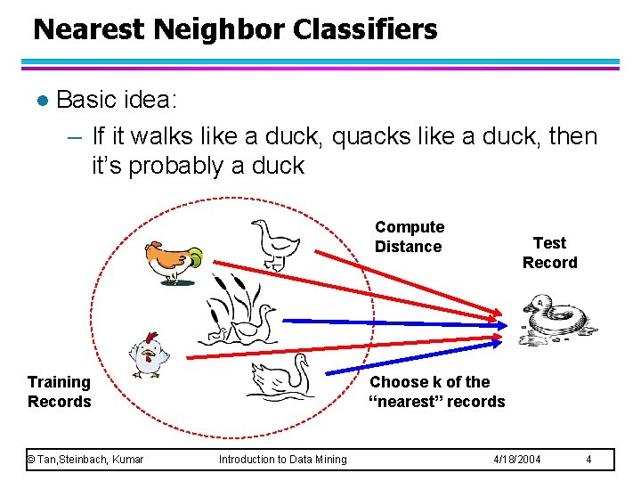
Nearest Neighbor Classifiers l Basic idea: – If it walks like a duck, quacks like a duck, then it’s probably a duck Compute Distance Training Records © Tan, Steinbach, Kumar Test Record Choose k of the “nearest” records Introduction to Data Mining 4/18/2004 4

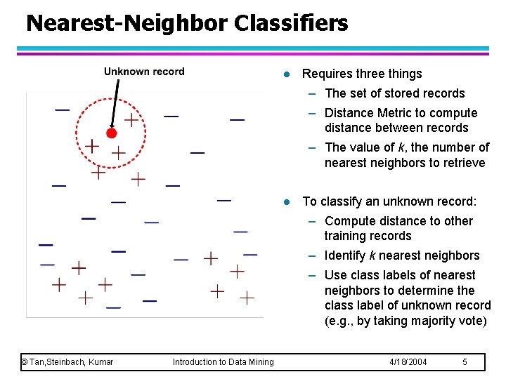
Nearest-Neighbor Classifiers l Requires three things – The set of stored records – Distance Metric to compute distance between records – The value of k, the number of nearest neighbors to retrieve l To classify an unknown record: – Compute distance to other training records – Identify k nearest neighbors – Use class labels of nearest neighbors to determine the class label of unknown record (e. g. , by taking majority vote) © Tan, Steinbach, Kumar Introduction to Data Mining 4/18/2004 5

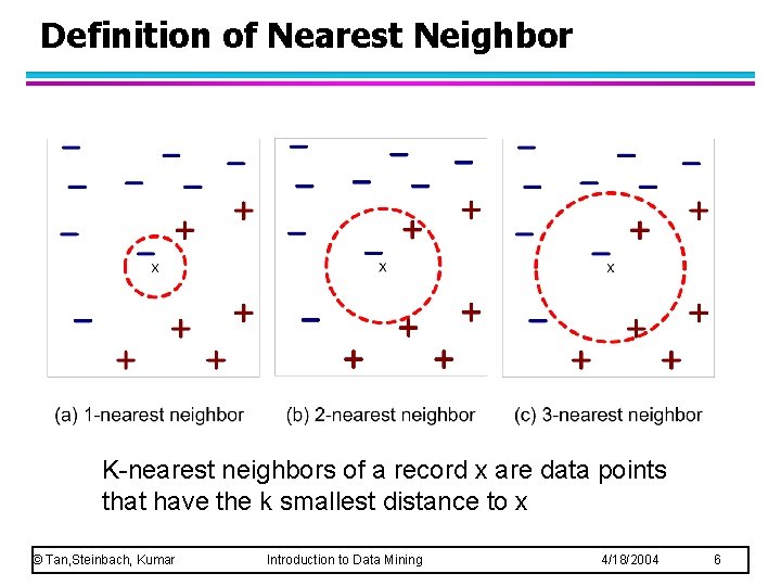
Definition of Nearest Neighbor K-nearest neighbors of a record x are data points that have the k smallest distance to x © Tan, Steinbach, Kumar Introduction to Data Mining 4/18/2004 6

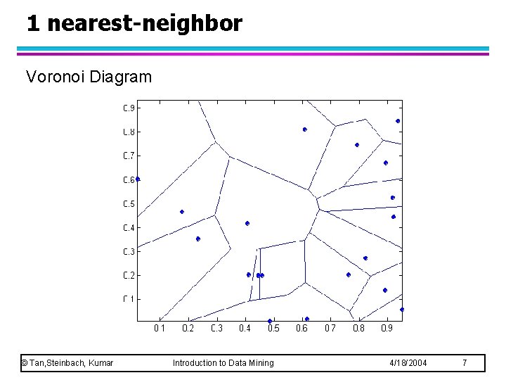
1 nearest-neighbor Voronoi Diagram © Tan, Steinbach, Kumar Introduction to Data Mining 4/18/2004 7

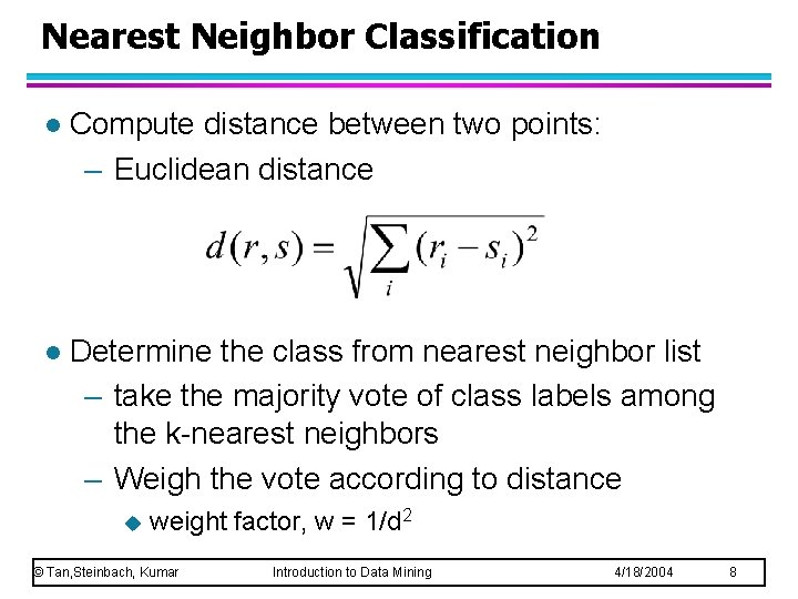
Nearest Neighbor Classification l Compute distance between two points: – Euclidean distance l Determine the class from nearest neighbor list – take the majority vote of class labels among the k-nearest neighbors – Weigh the vote according to distance u weight factor, w = 1/d 2 © Tan, Steinbach, Kumar Introduction to Data Mining 4/18/2004 8

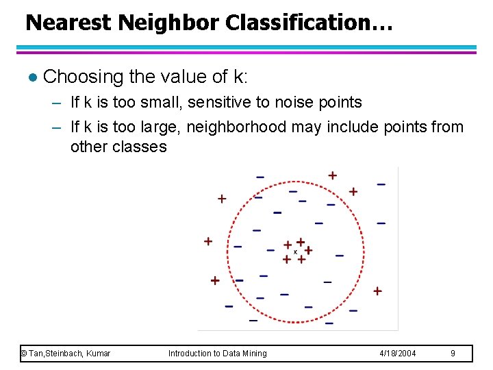
Nearest Neighbor Classification… l Choosing the value of k: – If k is too small, sensitive to noise points – If k is too large, neighborhood may include points from other classes © Tan, Steinbach, Kumar Introduction to Data Mining 4/18/2004 9

Nearest Neighbor Classification… l Scaling issues – Attributes may have to be scaled to prevent distance measures from being dominated by one of the attributes – Example: height of a person may vary from 1. 5 m to 1. 8 m u weight of a person may vary from 90 lb to 300 lb u income of a person may vary from $10 K to $1 M u © Tan, Steinbach, Kumar Introduction to Data Mining 4/18/2004 10

Nearest Neighbor Classification… l Problem with Euclidean measure: – High dimensional data u curse of dimensionality u Solution: Normalize the vectors to unit length © Tan, Steinbach, Kumar Introduction to Data Mining 4/18/2004 11

Nearest neighbor Classification… l k-NN classifiers are lazy learners – It does not build models explicitly – Unlike eager learners such as decision tree induction and rule-based systems – Classifying unknown records are relatively expensive © Tan, Steinbach, Kumar Introduction to Data Mining 4/18/2004 12

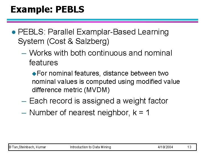
Example: PEBLS l PEBLS: Parallel Examplar-Based Learning System (Cost & Salzberg) – Works with both continuous and nominal features u. For nominal features, distance between two nominal values is computed using modified value difference metric (MVDM) – Each record is assigned a weight factor – Number of nearest neighbor, k = 1 © Tan, Steinbach, Kumar Introduction to Data Mining 4/18/2004 13

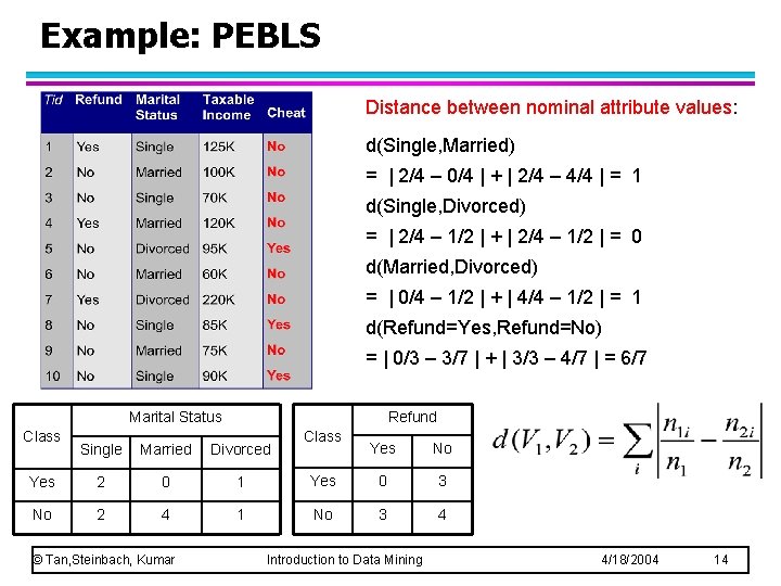
Example: PEBLS Distance between nominal attribute values: d(Single, Married) = | 2/4 – 0/4 | + | 2/4 – 4/4 | = 1 d(Single, Divorced) = | 2/4 – 1/2 | + | 2/4 – 1/2 | = 0 d(Married, Divorced) = | 0/4 – 1/2 | + | 4/4 – 1/2 | = 1 d(Refund=Yes, Refund=No) = | 0/3 – 3/7 | + | 3/3 – 4/7 | = 6/7 Marital Status Class Refund Single Married Divorced Yes 2 0 1 No 2 4 1 © Tan, Steinbach, Kumar Class Yes No Yes 0 3 No 3 4 Introduction to Data Mining 4/18/2004 14

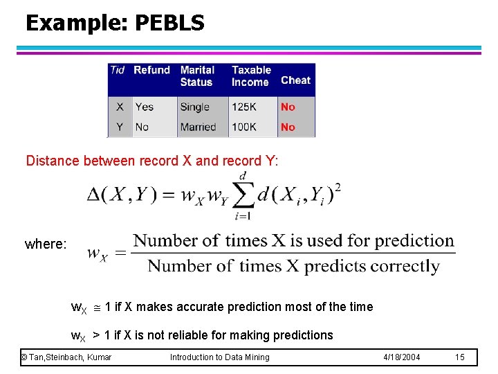
Example: PEBLS Distance between record X and record Y: where: w. X 1 if X makes accurate prediction most of the time w. X > 1 if X is not reliable for making predictions © Tan, Steinbach, Kumar Introduction to Data Mining 4/18/2004 15

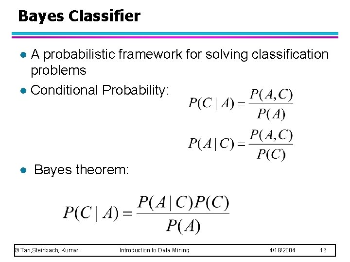
Bayes Classifier A probabilistic framework for solving classification problems l Conditional Probability: l l Bayes theorem: © Tan, Steinbach, Kumar Introduction to Data Mining 4/18/2004 16

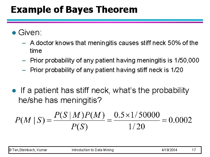
Example of Bayes Theorem l Given: – A doctor knows that meningitis causes stiff neck 50% of the time – Prior probability of any patient having meningitis is 1/50, 000 – Prior probability of any patient having stiff neck is 1/20 l If a patient has stiff neck, what’s the probability he/she has meningitis? © Tan, Steinbach, Kumar Introduction to Data Mining 4/18/2004 17

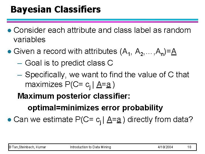
Bayesian Classifiers Consider each attribute and class label as random variables l Given a record with attributes (A 1, A 2, …, An)=A – Goal is to predict class C – Specifically, we want to find the value of C that maximizes P(C= cj | A=a ) Maximum posterior classifier: optimal=minimizes error probability l Can we estimate P(C= cj | A=a ) directly from data? l © Tan, Steinbach, Kumar Introduction to Data Mining 4/18/2004 18

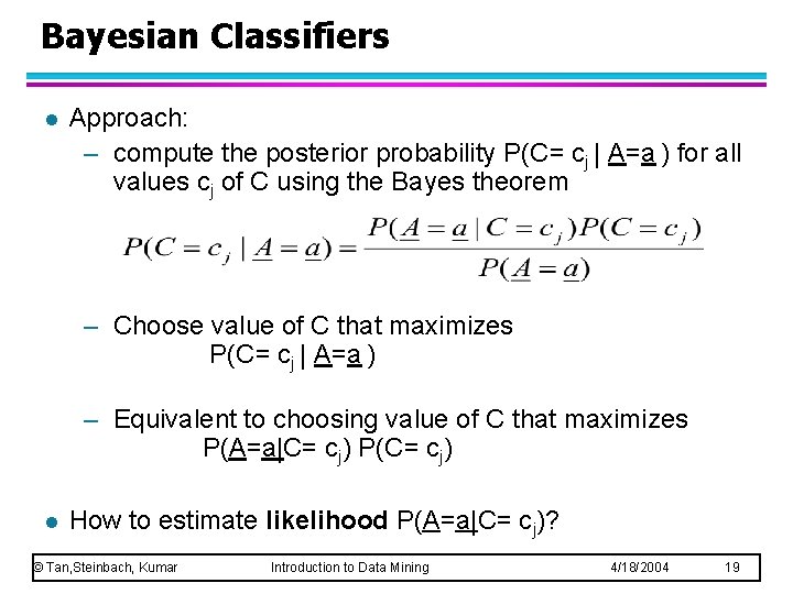
Bayesian Classifiers l Approach: – compute the posterior probability P(C= cj | A=a ) for all values cj of C using the Bayes theorem – Choose value of C that maximizes P(C= cj | A=a ) – Equivalent to choosing value of C that maximizes P(A=a|C= cj) P(C= cj) l How to estimate likelihood P(A=a|C= cj)? © Tan, Steinbach, Kumar Introduction to Data Mining 4/18/2004 19

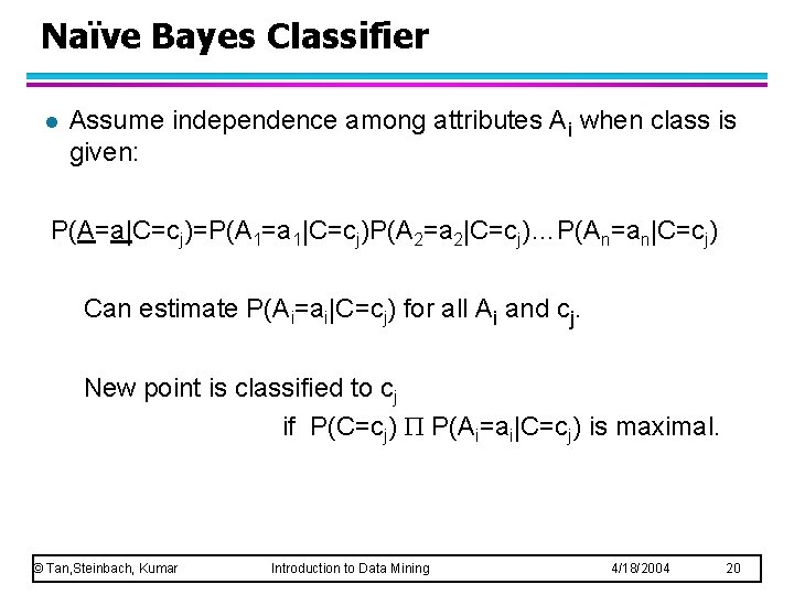
Naïve Bayes Classifier l Assume independence among attributes Ai when class is given: P(A=a|C=cj)=P(A 1=a 1|C=cj)P(A 2=a 2|C=cj)…P(An=an|C=cj) Can estimate P(Ai=ai|C=cj) for all Ai and cj. New point is classified to cj if P(C=cj) P(Ai=ai|C=cj) is maximal. © Tan, Steinbach, Kumar Introduction to Data Mining 4/18/2004 20

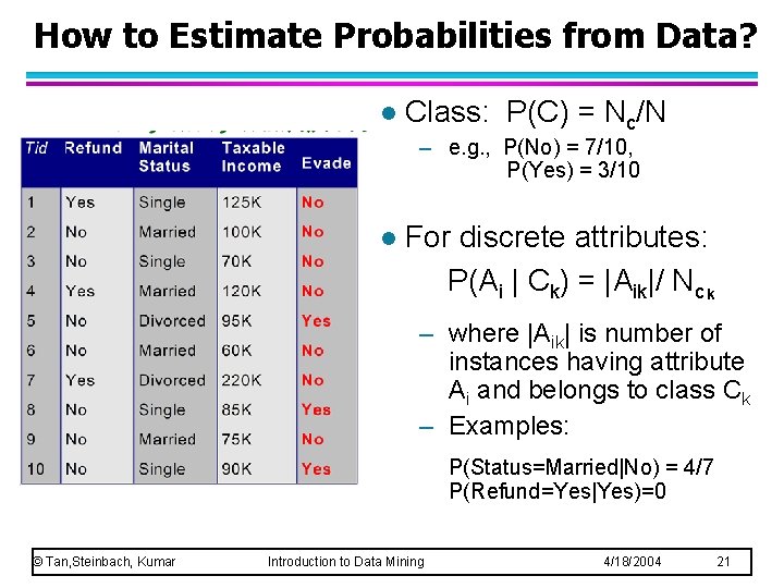
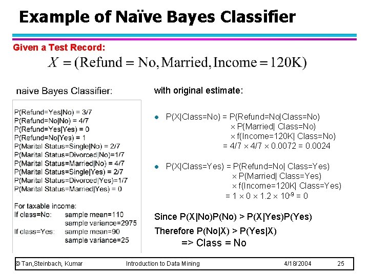
How to Estimate Probabilities from Data? l Class: P(C) = Nc/N – e. g. , P(No) = 7/10, P(Yes) = 3/10 l For discrete attributes: P(Ai | Ck) = |Aik|/ Nc k – where |Aik| is number of instances having attribute Ai and belongs to class Ck – Examples: P(Status=Married|No) = 4/7 P(Refund=Yes|Yes)=0 © Tan, Steinbach, Kumar Introduction to Data Mining 4/18/2004 21

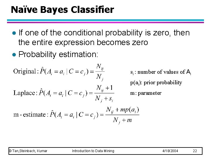
Naïve Bayes Classifier If one of the conditional probability is zero, then the entire expression becomes zero l Probability estimation: l si : number of values of Ai p(ai): prior probability m: parameter © Tan, Steinbach, Kumar Introduction to Data Mining 4/18/2004 22

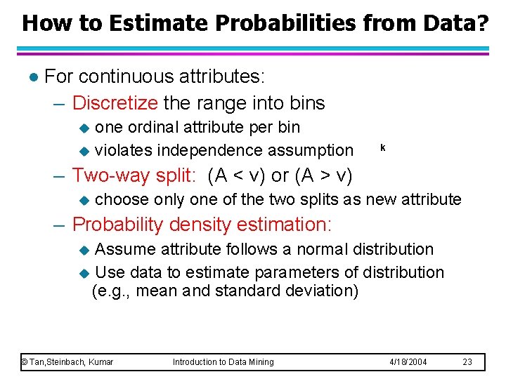
How to Estimate Probabilities from Data? l For continuous attributes: – Discretize the range into bins one ordinal attribute per bin u violates independence assumption u k – Two-way split: (A < v) or (A > v) u choose only one of the two splits as new attribute – Probability density estimation: Assume attribute follows a normal distribution u Use data to estimate parameters of distribution (e. g. , mean and standard deviation) u © Tan, Steinbach, Kumar Introduction to Data Mining 4/18/2004 23

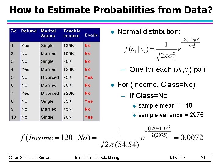
How to Estimate Probabilities from Data? l Normal distribution: – One for each (Ai, cj) pair l © Tan, Steinbach, Kumar For (Income, Class=No): – If Class=No Introduction to Data Mining u sample mean = 110 u sample variance = 2975 4/18/2004 24

Example of Naïve Bayes Classifier Given a Test Record: with original estimate: l P(X|Class=No) = P(Refund=No|Class=No) P(Married| Class=No) f(Income=120 K| Class=No) = 4/7 0. 0072 = 0. 0024 l P(X|Class=Yes) = P(Refund=No| Class=Yes) P(Married| Class=Yes) f(Income=120 K| Class=Yes) = 1 0 1. 2 10 -9 = 0 Since P(X|No)P(No) > P(X|Yes)P(Yes) Therefore P(No|X) > P(Yes|X) => Class = No © Tan, Steinbach, Kumar Introduction to Data Mining 4/18/2004 25

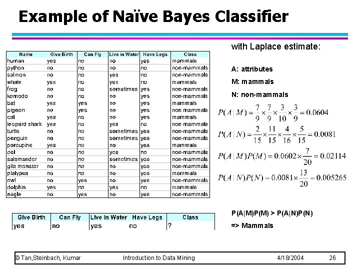
Example of Naïve Bayes Classifier with Laplace estimate: A: attributes M: mammals N: non-mammals P(A|M)P(M) > P(A|N)P(N) => Mammals © Tan, Steinbach, Kumar Introduction to Data Mining 4/18/2004 26

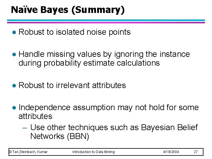
Naïve Bayes (Summary) l Robust to isolated noise points l Handle missing values by ignoring the instance during probability estimate calculations l Robust to irrelevant attributes l Independence assumption may not hold for some attributes – Use other techniques such as Bayesian Belief Networks (BBN) © Tan, Steinbach, Kumar Introduction to Data Mining 4/18/2004 27

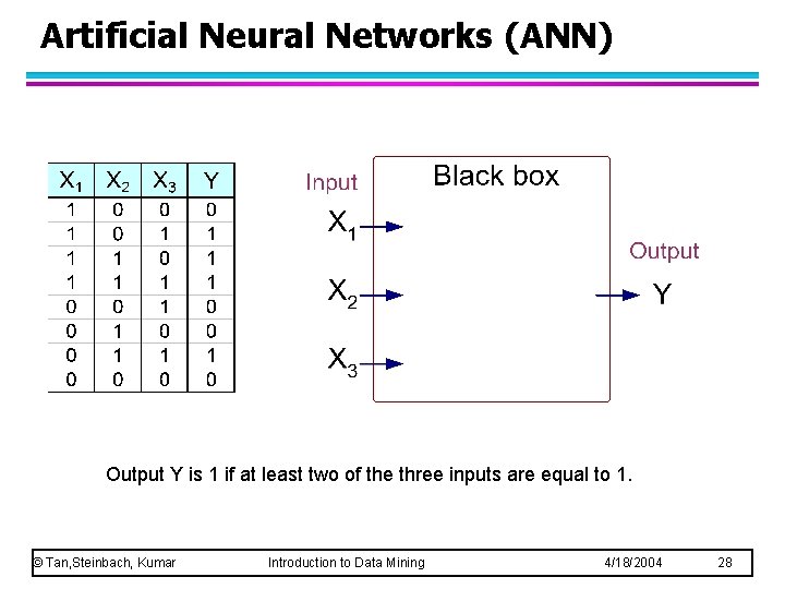
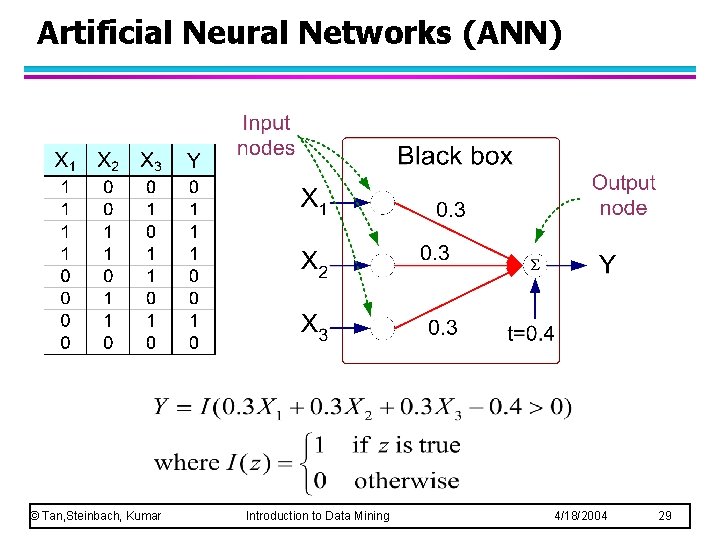
Artificial Neural Networks (ANN) Output Y is 1 if at least two of the three inputs are equal to 1. © Tan, Steinbach, Kumar Introduction to Data Mining 4/18/2004 28

Artificial Neural Networks (ANN) © Tan, Steinbach, Kumar Introduction to Data Mining 4/18/2004 29

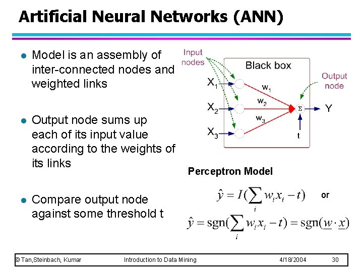
Artificial Neural Networks (ANN) l Model is an assembly of inter-connected nodes and weighted links l Output node sums up each of its input value according to the weights of its links l Perceptron Model or Compare output node against some threshold t © Tan, Steinbach, Kumar Introduction to Data Mining 4/18/2004 30

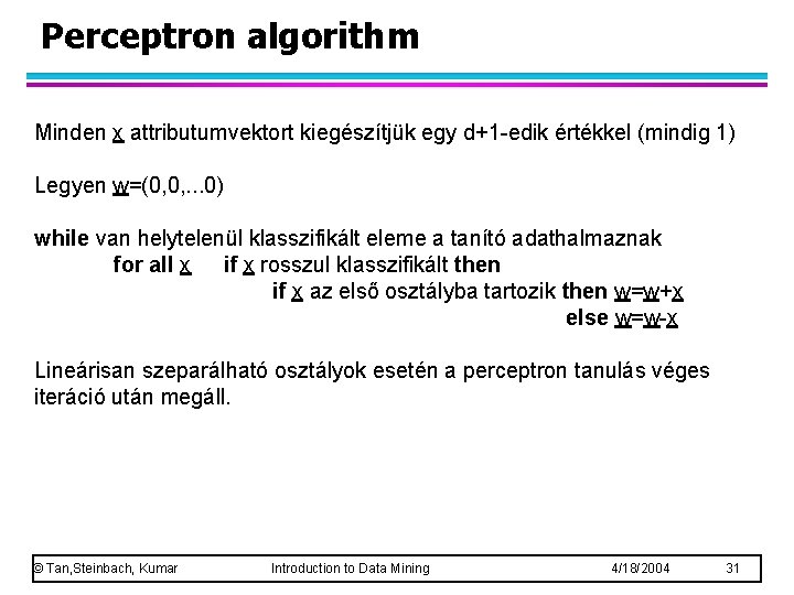
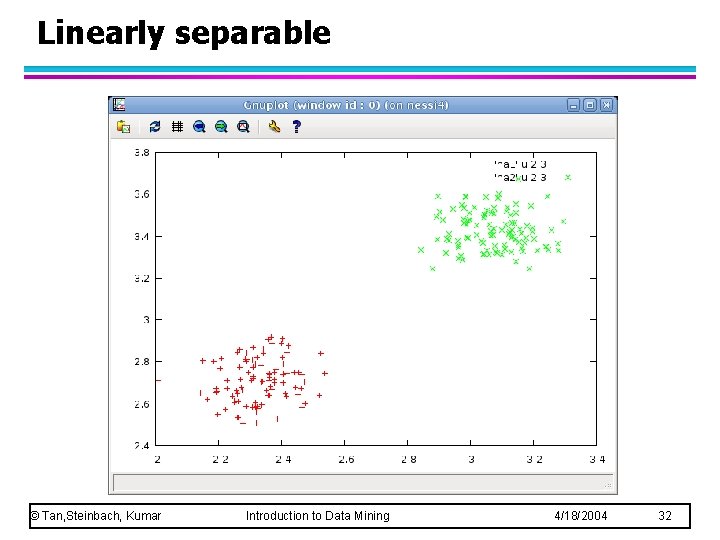
Perceptron algorithm Minden x attributumvektort kiegészítjük egy d+1 -edik értékkel (mindig 1) Legyen w=(0, 0, . . . 0) while van helytelenül klasszifikált eleme a tanító adathalmaznak for all x if x rosszul klasszifikált then if x az első osztályba tartozik then w=w+x else w=w-x Lineárisan szeparálható osztályok esetén a perceptron tanulás véges iteráció után megáll. © Tan, Steinbach, Kumar Introduction to Data Mining 4/18/2004 31

Linearly separable © Tan, Steinbach, Kumar Introduction to Data Mining 4/18/2004 32

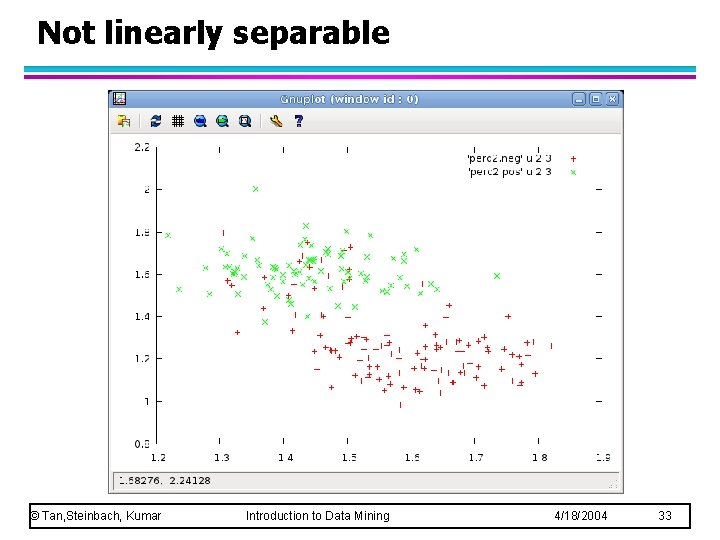
Not linearly separable © Tan, Steinbach, Kumar Introduction to Data Mining 4/18/2004 33

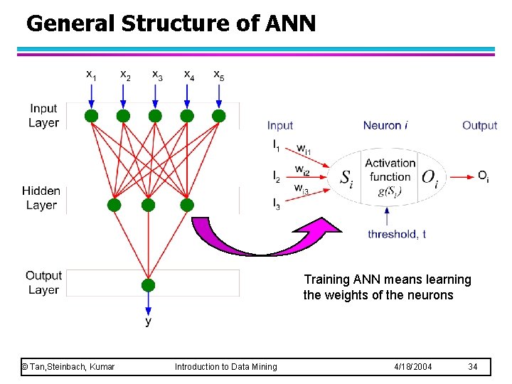
General Structure of ANN Training ANN means learning the weights of the neurons © Tan, Steinbach, Kumar Introduction to Data Mining 4/18/2004 34

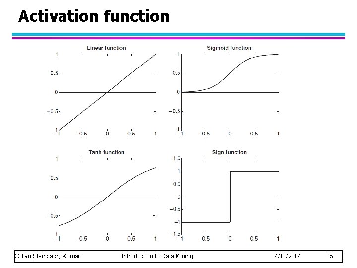
Activation function © Tan, Steinbach, Kumar Introduction to Data Mining 4/18/2004 35

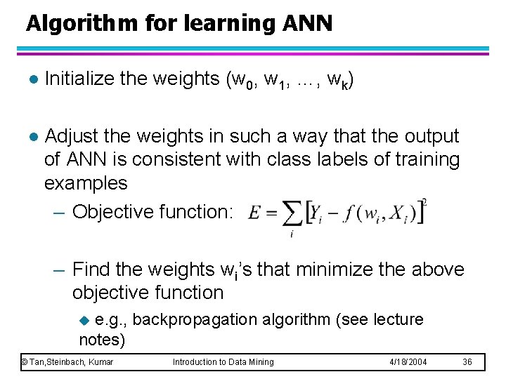
Algorithm for learning ANN l Initialize the weights (w 0, w 1, …, wk) l Adjust the weights in such a way that the output of ANN is consistent with class labels of training examples – Objective function: – Find the weights wi’s that minimize the above objective function e. g. , backpropagation algorithm (see lecture notes) u © Tan, Steinbach, Kumar Introduction to Data Mining 4/18/2004 36

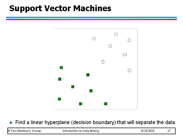
Support Vector Machines l Find a linear hyperplane (decision boundary) that will separate the data © Tan, Steinbach, Kumar Introduction to Data Mining 4/18/2004 37

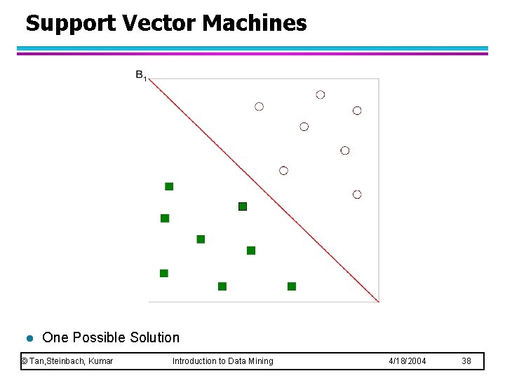
Support Vector Machines l One Possible Solution © Tan, Steinbach, Kumar Introduction to Data Mining 4/18/2004 38

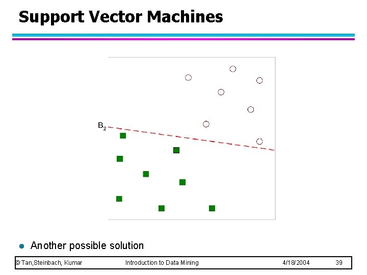
Support Vector Machines l Another possible solution © Tan, Steinbach, Kumar Introduction to Data Mining 4/18/2004 39

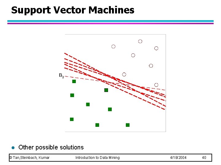
Support Vector Machines l Other possible solutions © Tan, Steinbach, Kumar Introduction to Data Mining 4/18/2004 40

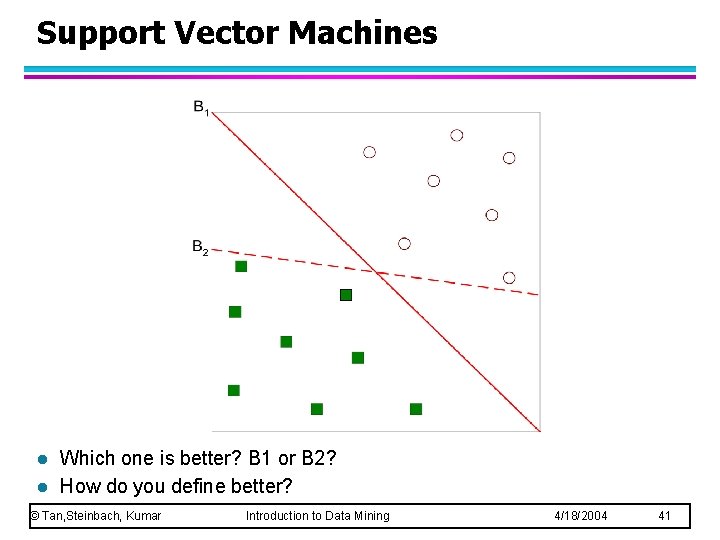
Support Vector Machines l l Which one is better? B 1 or B 2? How do you define better? © Tan, Steinbach, Kumar Introduction to Data Mining 4/18/2004 41

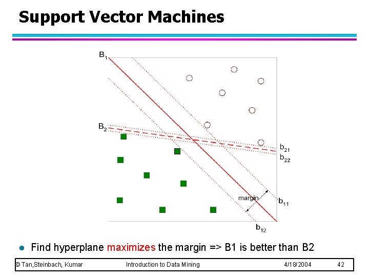
Support Vector Machines l Find hyperplane maximizes the margin => B 1 is better than B 2 © Tan, Steinbach, Kumar Introduction to Data Mining 4/18/2004 42

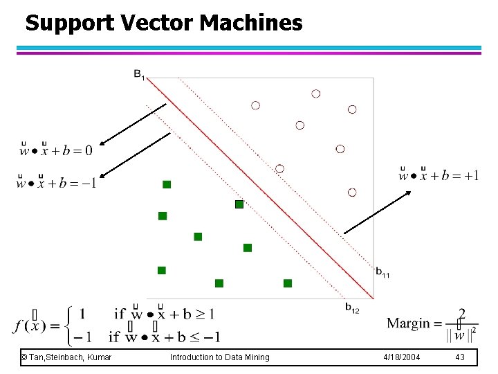
Support Vector Machines © Tan, Steinbach, Kumar Introduction to Data Mining 4/18/2004 43

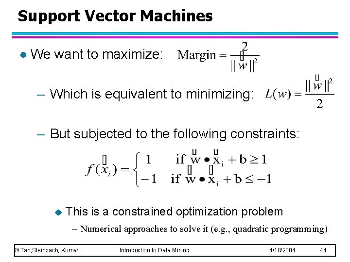
Support Vector Machines l We want to maximize: – Which is equivalent to minimizing: – But subjected to the following constraints: u This is a constrained optimization problem – Numerical approaches to solve it (e. g. , quadratic programming) © Tan, Steinbach, Kumar Introduction to Data Mining 4/18/2004 44

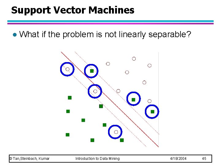
Support Vector Machines l What if the problem is not linearly separable? © Tan, Steinbach, Kumar Introduction to Data Mining 4/18/2004 45

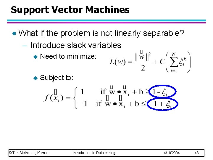
Support Vector Machines l What if the problem is not linearly separable? – Introduce slack variables u Need to minimize: u Subject to: © Tan, Steinbach, Kumar Introduction to Data Mining 4/18/2004 46

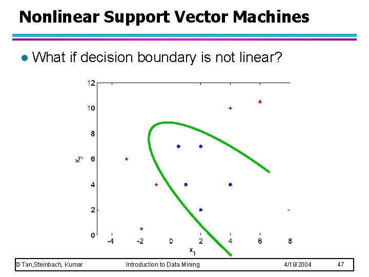
Nonlinear Support Vector Machines l What if decision boundary is not linear? © Tan, Steinbach, Kumar Introduction to Data Mining 4/18/2004 47

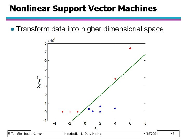
Nonlinear Support Vector Machines l Transform data into higher dimensional space © Tan, Steinbach, Kumar Introduction to Data Mining 4/18/2004 48

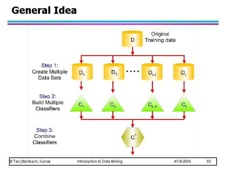
Ensemble Methods l Construct a set of classifiers from the training data l Predict class label of previously unseen records by aggregating predictions made by multiple classifiers © Tan, Steinbach, Kumar Introduction to Data Mining 4/18/2004 49

General Idea © Tan, Steinbach, Kumar Introduction to Data Mining 4/18/2004 50

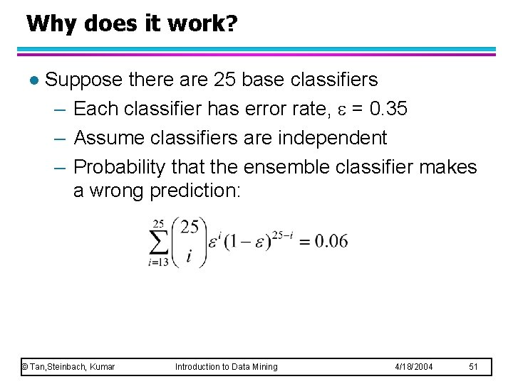
Why does it work? l Suppose there are 25 base classifiers – Each classifier has error rate, = 0. 35 – Assume classifiers are independent – Probability that the ensemble classifier makes a wrong prediction: © Tan, Steinbach, Kumar Introduction to Data Mining 4/18/2004 51

Examples of Ensemble Methods l How to generate an ensemble of classifiers? – Bagging – Boosting © Tan, Steinbach, Kumar Introduction to Data Mining 4/18/2004 52

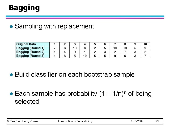
Bagging l Sampling with replacement l Build classifier on each bootstrap sample l Each sample has probability (1 – 1/n)n of being selected © Tan, Steinbach, Kumar Introduction to Data Mining 4/18/2004 53

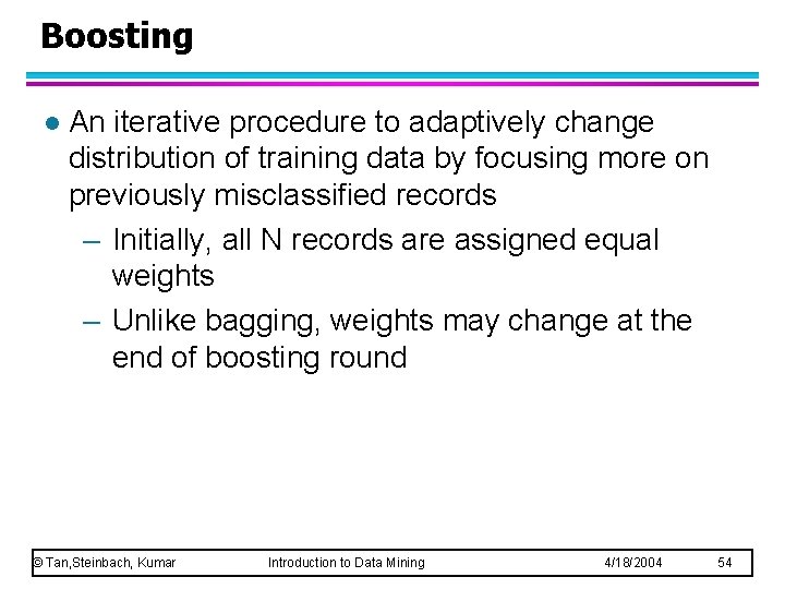
Boosting l An iterative procedure to adaptively change distribution of training data by focusing more on previously misclassified records – Initially, all N records are assigned equal weights – Unlike bagging, weights may change at the end of boosting round © Tan, Steinbach, Kumar Introduction to Data Mining 4/18/2004 54

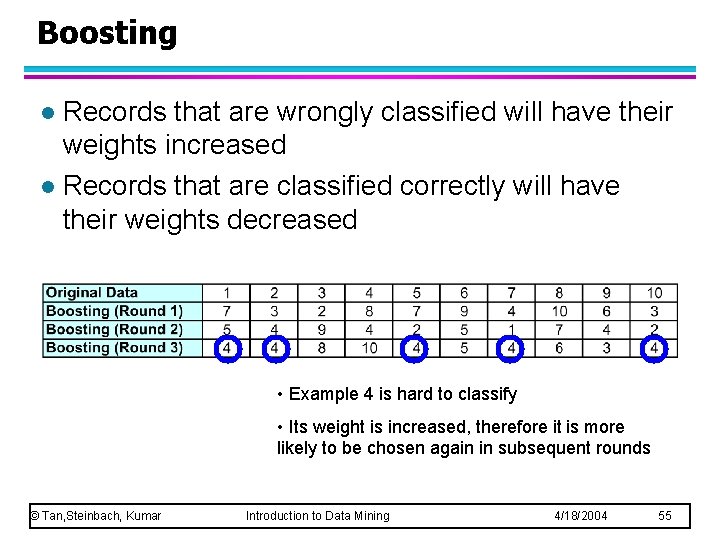
Boosting Records that are wrongly classified will have their weights increased l Records that are classified correctly will have their weights decreased l • Example 4 is hard to classify • Its weight is increased, therefore it is more likely to be chosen again in subsequent rounds © Tan, Steinbach, Kumar Introduction to Data Mining 4/18/2004 55

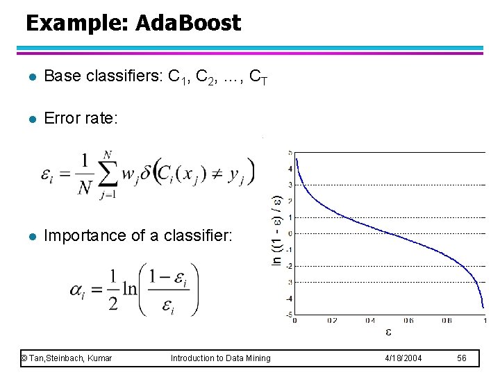
Example: Ada. Boost l Base classifiers: C 1, C 2, …, CT l Error rate: l Importance of a classifier: © Tan, Steinbach, Kumar Introduction to Data Mining 4/18/2004 56

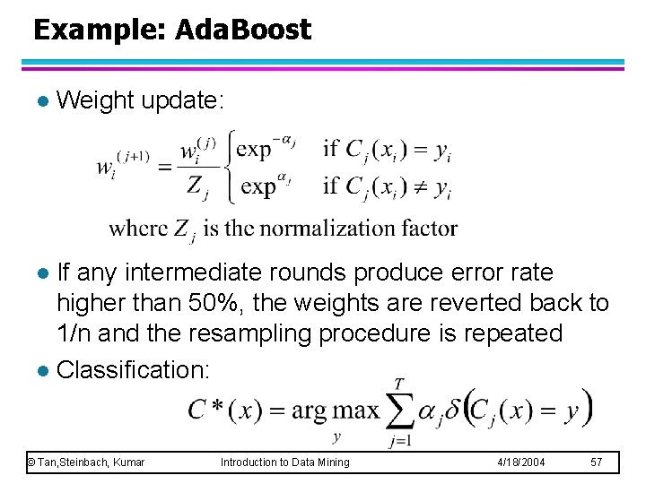
Example: Ada. Boost l Weight update: If any intermediate rounds produce error rate higher than 50%, the weights are reverted back to 1/n and the resampling procedure is repeated l Classification: l © Tan, Steinbach, Kumar Introduction to Data Mining 4/18/2004 57

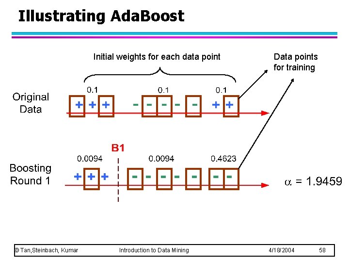
Illustrating Ada. Boost Initial weights for each data point © Tan, Steinbach, Kumar Introduction to Data Mining Data points for training 4/18/2004 58

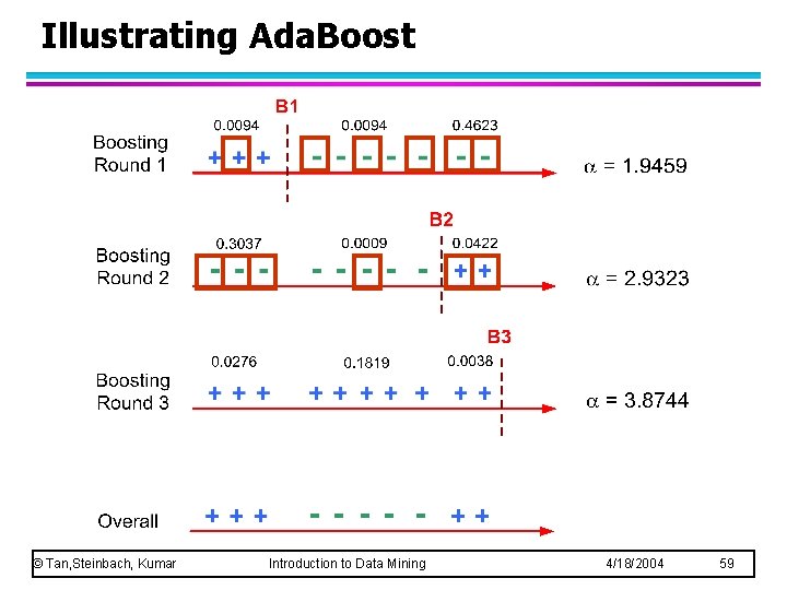
Illustrating Ada. Boost © Tan, Steinbach, Kumar Introduction to Data Mining 4/18/2004 59