Data Mining Classification Alternative Techniques From Chapter 5

Data Mining Classification: Alternative Techniques From Chapter 5 in Introduction to Data Mining by Tan, Steinbach, Kumar

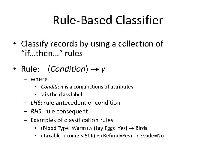
Rule-Based Classifier • Classify records by using a collection of “if…then…” rules • Rule: (Condition) y – where • Condition is a conjunctions of attributes • y is the class label – LHS: rule antecedent or condition – RHS: rule consequent – Examples of classification rules: • (Blood Type=Warm) (Lay Eggs=Yes) Birds • (Taxable Income < 50 K) (Refund=Yes) Evade=No

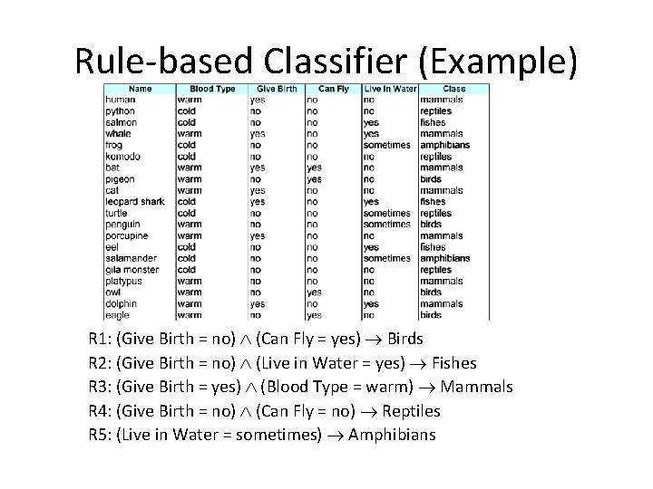
Rule-based Classifier (Example) R 1: (Give Birth = no) (Can Fly = yes) Birds R 2: (Give Birth = no) (Live in Water = yes) Fishes R 3: (Give Birth = yes) (Blood Type = warm) Mammals R 4: (Give Birth = no) (Can Fly = no) Reptiles R 5: (Live in Water = sometimes) Amphibians

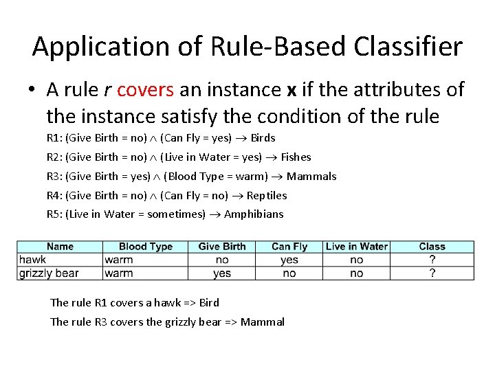
Application of Rule-Based Classifier • A rule r covers an instance x if the attributes of the instance satisfy the condition of the rule R 1: (Give Birth = no) (Can Fly = yes) Birds R 2: (Give Birth = no) (Live in Water = yes) Fishes R 3: (Give Birth = yes) (Blood Type = warm) Mammals R 4: (Give Birth = no) (Can Fly = no) Reptiles R 5: (Live in Water = sometimes) Amphibians The rule R 1 covers a hawk => Bird The rule R 3 covers the grizzly bear => Mammal

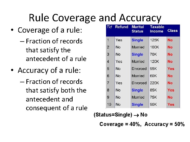
Rule Coverage and Accuracy • Coverage of a rule: – Fraction of records that satisfy the antecedent of a rule • Accuracy of a rule: – Fraction of records that satisfy both the antecedent and consequent of a rule (Status=Single) No Coverage = 40%, Accuracy = 50%

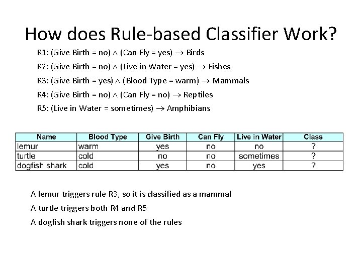
How does Rule-based Classifier Work? R 1: (Give Birth = no) (Can Fly = yes) Birds R 2: (Give Birth = no) (Live in Water = yes) Fishes R 3: (Give Birth = yes) (Blood Type = warm) Mammals R 4: (Give Birth = no) (Can Fly = no) Reptiles R 5: (Live in Water = sometimes) Amphibians A lemur triggers rule R 3, so it is classified as a mammal A turtle triggers both R 4 and R 5 A dogfish shark triggers none of the rules

Characteristics of Rule-Based Classifier • Mutually exclusive rules – Classifier contains mutually exclusive rules if the rules are independent of each other – Every record is covered by at most one rule • Exhaustive rules – Classifier has exhaustive coverage if it accounts for every possible combination of attribute values – Each record is covered by at least one rule

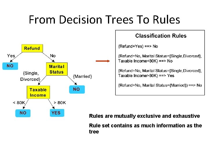
From Decision Trees To Rules are mutually exclusive and exhaustive Rule set contains as much information as the tree

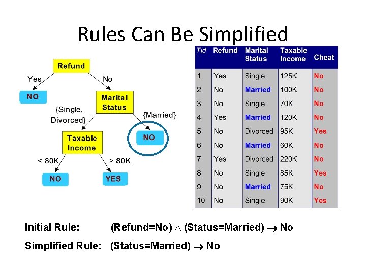
Rules Can Be Simplified Initial Rule: (Refund=No) (Status=Married) No Simplified Rule: (Status=Married) No

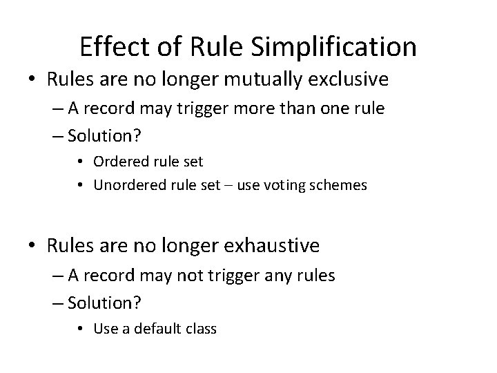
Effect of Rule Simplification • Rules are no longer mutually exclusive – A record may trigger more than one rule – Solution? • Ordered rule set • Unordered rule set – use voting schemes • Rules are no longer exhaustive – A record may not trigger any rules – Solution? • Use a default class

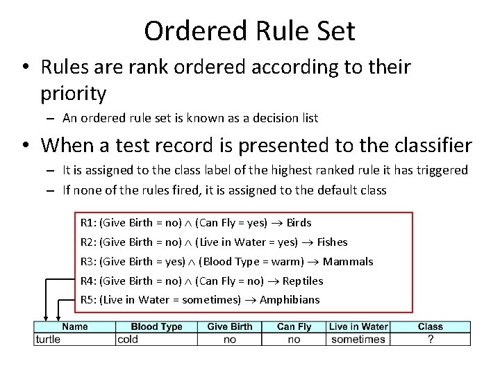
Ordered Rule Set • Rules are rank ordered according to their priority – An ordered rule set is known as a decision list • When a test record is presented to the classifier – It is assigned to the class label of the highest ranked rule it has triggered – If none of the rules fired, it is assigned to the default class R 1: (Give Birth = no) (Can Fly = yes) Birds R 2: (Give Birth = no) (Live in Water = yes) Fishes R 3: (Give Birth = yes) (Blood Type = warm) Mammals R 4: (Give Birth = no) (Can Fly = no) Reptiles R 5: (Live in Water = sometimes) Amphibians

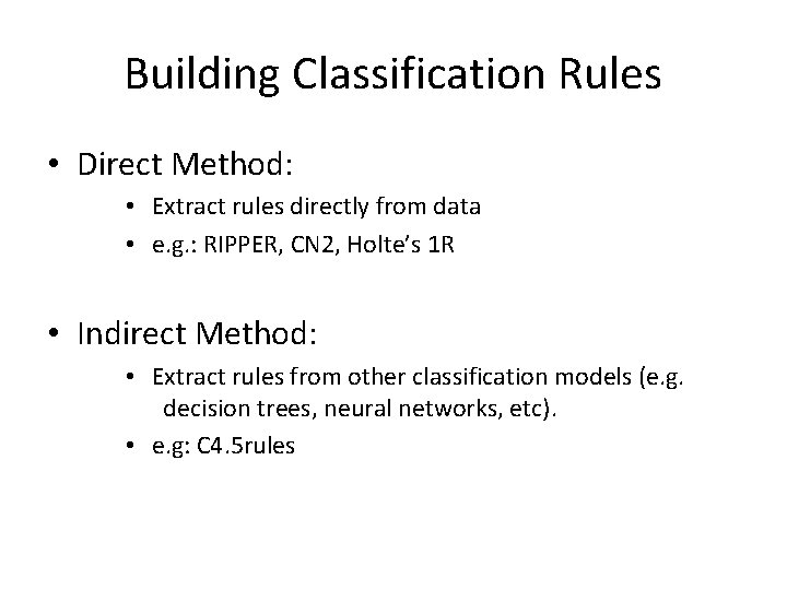
Building Classification Rules • Direct Method: • Extract rules directly from data • e. g. : RIPPER, CN 2, Holte’s 1 R • Indirect Method: • Extract rules from other classification models (e. g. decision trees, neural networks, etc). • e. g: C 4. 5 rules

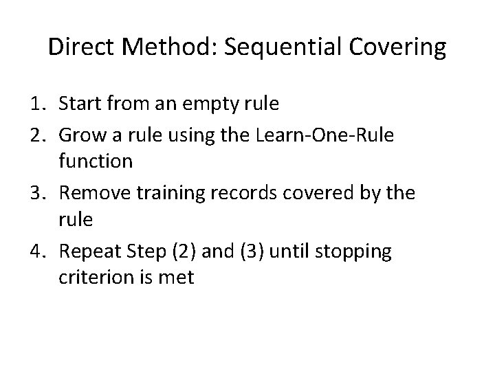
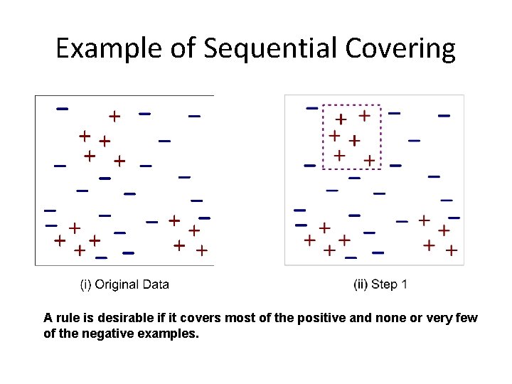
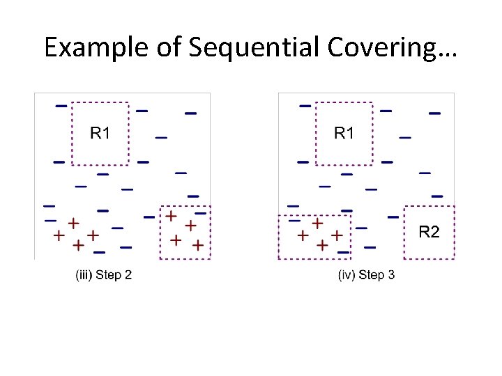
Direct Method: Sequential Covering 1. Start from an empty rule 2. Grow a rule using the Learn-One-Rule function 3. Remove training records covered by the rule 4. Repeat Step (2) and (3) until stopping criterion is met

Example of Sequential Covering A rule is desirable if it covers most of the positive and none or very few of the negative examples.

Example of Sequential Covering…

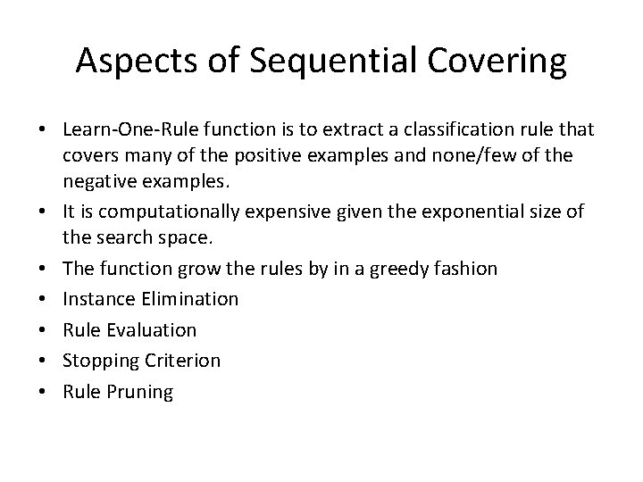
Aspects of Sequential Covering • Learn-One-Rule function is to extract a classification rule that covers many of the positive examples and none/few of the negative examples. • It is computationally expensive given the exponential size of the search space. • The function grow the rules by in a greedy fashion • Instance Elimination • Rule Evaluation • Stopping Criterion • Rule Pruning

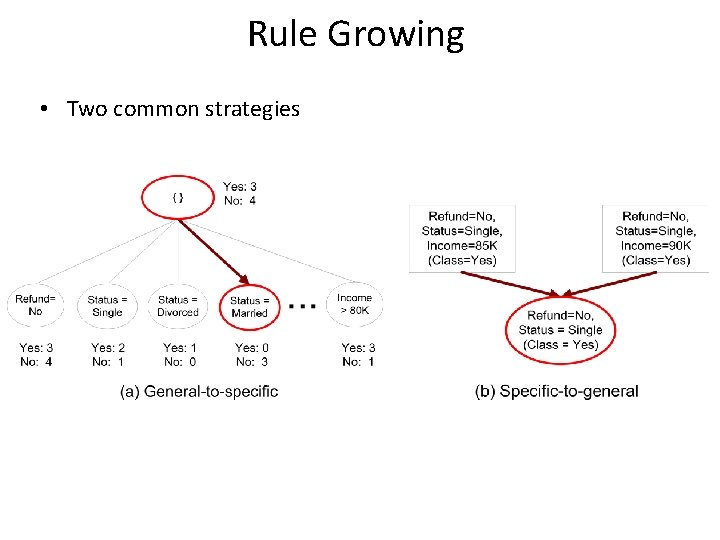
Rule Growing • Two common strategies

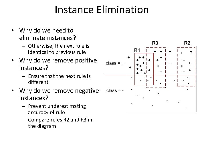
Instance Elimination • Why do we need to eliminate instances? – Otherwise, the next rule is identical to previous rule • Why do we remove positive instances? – Ensure that the next rule is different • Why do we remove negative instances? – Prevent underestimating accuracy of rule – Compare rules R 2 and R 3 in the diagram

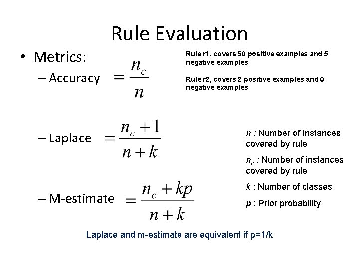
• Metrics: Rule Evaluation – Accuracy – Laplace Rule r 1, covers 50 positive examples and 5 negative examples Rule r 2, covers 2 positive examples and 0 negative examples n : Number of instances covered by rule nc : Number of instances covered by rule – M-estimate k : Number of classes p : Prior probability Laplace and m-estimate are equivalent if p=1/k

Stopping Criterion and Rule Pruning • Stopping criterion – Compute the gain – If gain is not significant, discard the new rule • Rule Pruning – Similar to post-pruning of decision trees – Reduced Error Pruning: • Remove one of the conjuncts in the rule • Compare error rate on validation set before and after pruning • If error improves, prune the conjunct

Summary of Direct Method • Grow a single rule • Remove Instances from rule • Prune the rule (if necessary) • Add rule to Current Rule Set • Repeat

Direct Method: RIPPER • For 2 -class problem, choose one of the classes as positive class, and the other as negative class – Learn rules for positive class – Negative class will be default class • For multi-class problem – Order the classes according to increasing class prevalence (fraction of instances that belong to a particular class) – Learn the rule set for smallest class first, treat the rest as negative class – Repeat with next smallest class as positive class

Direct Method: RIPPER • Growing a rule: – Start from empty rule – Add conjuncts as long as they improve FOIL’s information gain – Stop when rule no longer covers negative examples – Prune the rule immediately using incremental reduced error pruning – Measure for pruning: v = (p-n)/(p+n) • p: number of positive examples covered by the rule in the validation set • n: number of negative examples covered by the rule in the validation set – Pruning method: delete any final sequence of conditions that maximizes v

Direct Method: RIPPER • Building a Rule Set: – Use sequential covering algorithm • Finds the best rule that covers the current set of positive examples • Eliminate both positive and negative examples covered by the rule – Each time a rule is added to the rule set, compute the new description length • stop adding new rules when the new description length is d bits longer than the smallest description length obtained so far

Direct Method: RIPPER • Optimize the rule set: – For each rule r in the rule set R • Consider 2 alternative rules: – Replacement rule (r*): grow new rule from scratch – Revised rule(r’): add conjuncts to extend the rule r • Compare the rule set for r against the rule set for r* and r’ • Choose rule set that minimizes MDL principle – Repeat rule generation and rule optimization for the remaining positive examples

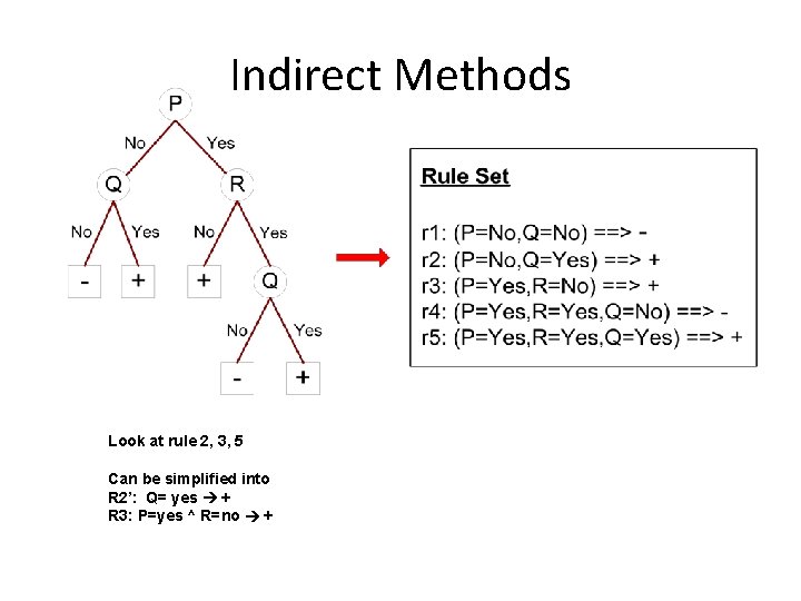
Indirect Methods Look at rule 2, 3, 5 Can be simplified into R 2’: Q= yes + R 3: P=yes ^ R=no +

Indirect Method: C 4. 5 rules • Extract rules from an unpruned decision tree • For each rule, r: A y, – consider an alternative rule r’: A’ y where A’ is obtained by removing one of the conjuncts in A – Compare the error rate for r against all r’s – Prune if one of the r’s has lower error rate – Repeat until we can no longer improve generalization error

Indirect Method: C 4. 5 rules • Instead of ordering the rules, order subsets of rules (class ordering) – Each subset is a collection of rules with the same rule consequent (class) – Compute description length of each subset • Description length = L(error) + g L(model) • g is a parameter that takes into account the presence of redundant attributes in a rule set (default value = 0. 5)

Advantages of Rule-Based Classifiers • • • As highly expressive as decision trees Easy to interpret Easy to generate Can classify new instances rapidly Performance comparable to decision trees