DATA MINING CLASS IMBALANCE Last modified 4319 1

DATA MINING CLASS IMBALANCE Last modified 4/3/19 1

Class Imbalance Problem Lots of classification problems where the classes are skewed (more records from one class than another) Credit card fraud Intrusion detection Telecommunication switching equipment failures 2

Challenges Evaluation measures such as accuracy are not well-suited for imbalanced class Prediction algorithms are generally focused on maximizing accuracy Detecting the rare class is like finding needle in a haystack 3

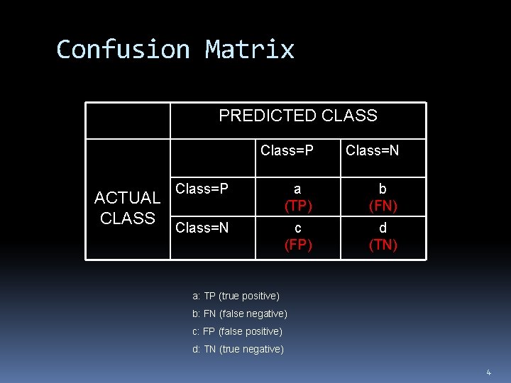
Confusion Matrix PREDICTED CLASS ACTUAL CLASS Class=P Class=N Class=P a (TP) b (FN) Class=N c (FP) d (TN) a: TP (true positive) b: FN (false negative) c: FP (false positive) d: TN (true negative) 4

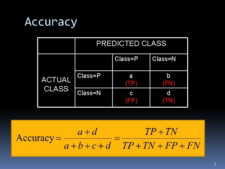
Accuracy PREDICTED CLASS ACTUAL CLASS Class=P Class=N Class=P a (TP) b (FN) Class=N c (FP) d (TN) 5

Problem with Accuracy Consider a 2 -class problem Number of Class NO examples = 990 Number of Class YES examples = 10 If a model predicts everything to be class NO, accuracy is 990/1000 = 99 % This is misleading because the model does not detect any class YES example Detecting the rare class is usually more interesting (e. g. , frauds, intrusions, defects, etc. ) Underlying issue is that the two classes are not equally important 6

Metrics Suited to Class Imbalance We need metrics tailored to class imbalance Note that if a metric treats all classes equally, then relatively speaking, the minority class counts for more than if accuracy is used For example, if we reported balanced accuracy, which is the average of the accuracy on each class, then the minority class would count as much as majority class, where normally they are weighted by the number of examples in each class Alternatively, we could have metrics that describe performance on the minority class 7

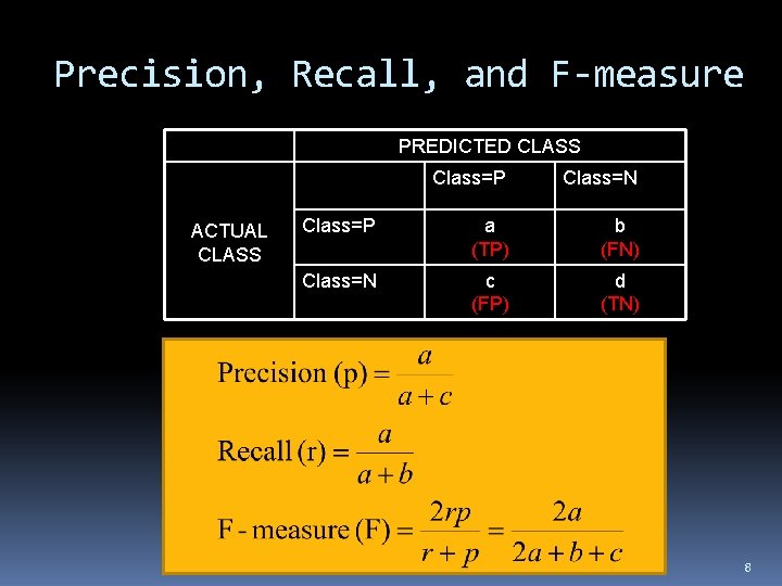
Precision, Recall, and F-measure PREDICTED CLASS ACTUAL CLASS Class=P Class=N Class=P a (TP) b (FN) Class=N c (FP) d (TN) 8

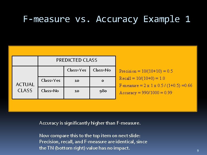
F-measure vs. Accuracy Example 1 PREDICTED CLASS ACTUAL CLASS Class=Yes Class=No Class=Yes 10 0 Class=No 10 980 Precision = 10/(10+10) = 0. 5 Recall = 10/(10+0) = 1. 0 F-measure = 2 x 1 x 0. 5 / (1+0. 5) =0. 66 Accuracy = 990/1000 = 0. 99 Accuracy is significantly higher than F-measure. Now compare this to the top item on next slide: Precision, recall, and F-measure are identical, since the TN (bottom right) value has no impact. 9

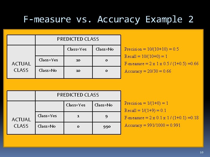
F-measure vs. Accuracy Example 2 PREDICTED CLASS Class=Yes ACTUAL CLASS Class=No Class=Yes 10 0 Class=No 10 0 Precision = 10/(10+10) = 0. 5 Recall = 10/(10+0) = 1 F-measure = 2 x 1 x 0. 5 / (1+0. 5) =0. 66 Accuracy = 20/30 = 0. 66 PREDICTED CLASS Class=Yes ACTUAL CLASS Class=No Class=Yes 1 9 Class=No 0 990 Precision = 1/(1+0) = 1 Recall = 1/(1+9) = 0. 1 F-measure = 2 x 0. 1 x 1 / (1+0. 1) =0. 18 Accuracy = 991/1000 = 0. 991 10

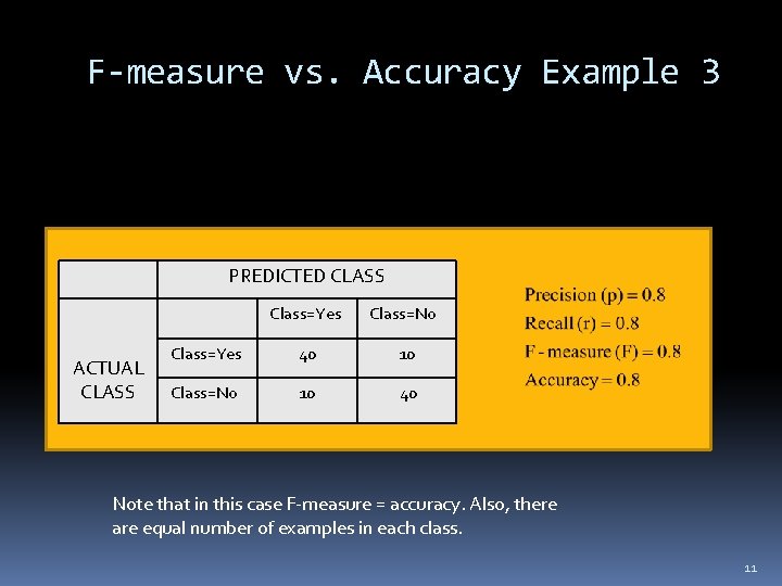
F-measure vs. Accuracy Example 3 PREDICTED CLASS ACTUAL CLASS Class=Yes Class=No Class=Yes 40 10 Class=No 10 40 Note that in this case F-measure = accuracy. Also, there are equal number of examples in each class. 11

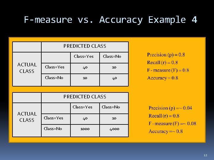
F-measure vs. Accuracy Example 4 PREDICTED CLASS Class=Yes ACTUAL CLASS Class=No Class=Yes 40 10 Class=No 10 40 PREDICTED CLASS Class=Yes ACTUAL CLASS Class=No Class=Yes 40 10 Class=No 1000 4000 12

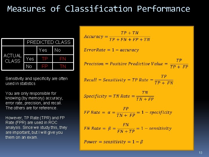
Measures of Classification Performance PREDICTED CLASS Yes ACTUAL Yes CLASS No No TP FN FP TN Sensitivity and specificity are often used in statistics You are only responsible for knowing (by memory) accuracy, error rate, precision, and recall. The others are for reference. However, TP Rate (TPR) and FP Rate (FPR) are used in ROC analysis. Since we study this, they are important, but I will give you them on an exam. 13

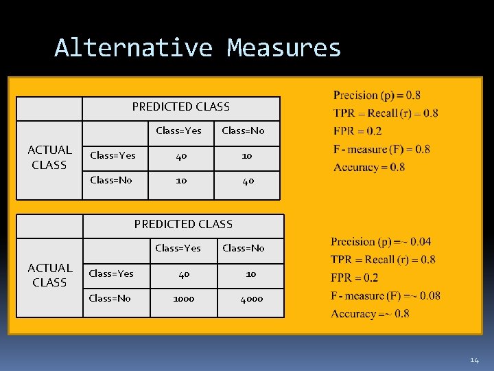
Alternative Measures PREDICTED CLASS Class=Yes ACTUAL CLASS Class=No Class=Yes 40 10 Class=No 10 40 PREDICTED CLASS Class=Yes ACTUAL CLASS Class=No Class=Yes 40 10 Class=No 1000 4000 14

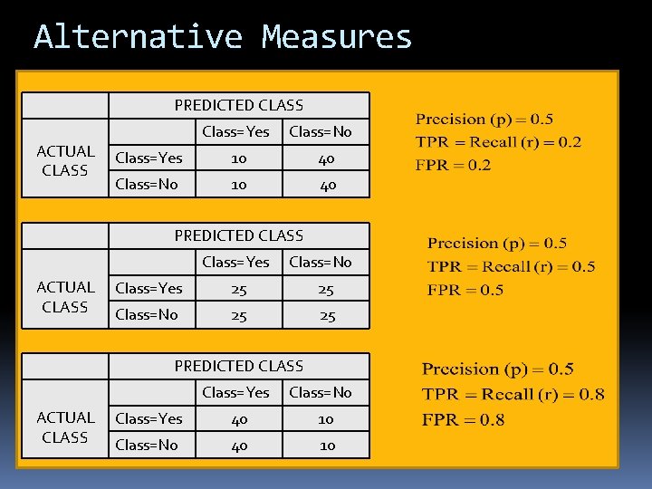
Alternative Measures PREDICTED CLASS ACTUAL CLASS Class=Yes Class=No Class=Yes 10 40 Class=No 10 40 PREDICTED CLASS Class=Yes ACTUAL CLASS Class=No Class=Yes 25 25 Class=No 25 25 PREDICTED CLASS Class=Yes ACTUAL CLASS Class=No Class=Yes 40 10 Class=No 40 10

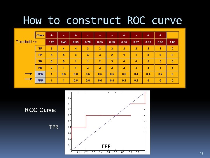
ROC (Receiver Operating Characteristic) A graphical approach for displaying trade-off between detection rate and false alarm rate Developed in 1950 s for signal detection theory to analyze noisy signals ROC curve plots TPR against FPR Performance of a model represented as a point in an ROC curve Changing the threshold parameter of classifier changes the location of the point 16

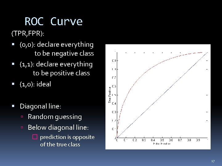
ROC Curve (TPR, FPR): (0, 0): declare everything to be negative class (1, 1): declare everything to be positive class (1, 0): ideal Diagonal line: Random guessing Below diagonal line: � prediction is opposite of the true class 17

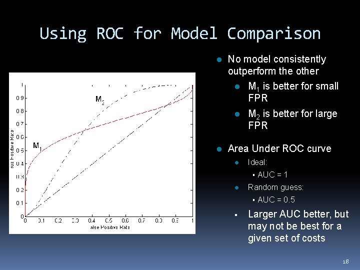
Using ROC for Model Comparison l l No model consistently outperform the other l M 1 is better for small FPR l M 2 is better for large FPR Area Under ROC curve l Ideal: l Random guess: AUC = 1 AUC = 0. 5 Larger AUC better, but may not be best for a given set of costs 18

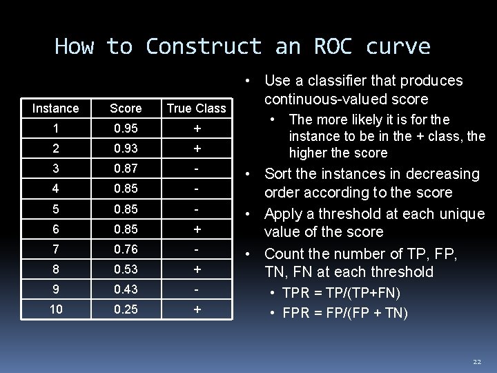
ROC Curve To draw ROC curve, classifier must produce continuous-valued output Outputs are used to rank test records, from the most likely positive class record to the least likely positive class record Many classifiers produce only discrete outputs (i. e. , predicted class) How to get continuous-valued outputs? � Decision trees, rule-based classifiers, neural networks, Bayesian classifiers, k-nearest neighbors, SVM 19

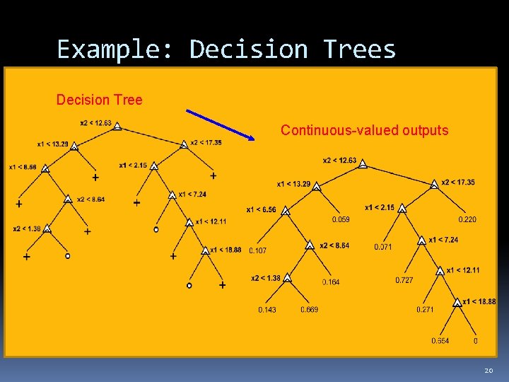
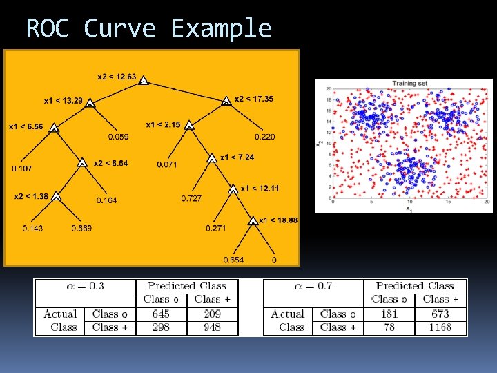
Example: Decision Trees Decision Tree Continuous-valued outputs 20

ROC Curve Example

How to Construct an ROC curve Instance Score True Class 1 0. 95 + 2 0. 93 + 3 0. 87 - 4 0. 85 - 5 0. 85 - 6 0. 85 + 7 0. 76 - 8 0. 53 + 9 0. 43 - 10 0. 25 + • Use a classifier that produces continuous-valued score • The more likely it is for the instance to be in the + class, the higher the score • Sort the instances in decreasing order according to the score • Apply a threshold at each unique value of the score • Count the number of TP, FP, TN, FN at each threshold • TPR = TP/(TP+FN) • FPR = FP/(FP + TN) 22

How to construct ROC curve Threshold >= ROC Curve: TPR FPR 23

Handling Class Imbalance Problem Class-based ordering (e. g. RIPPER) Rules for rare class have higher priority Cost-sensitive classification Misclassifying rare class as majority class is more expensive than misclassifying majority as rare class Sampling-based approaches 24

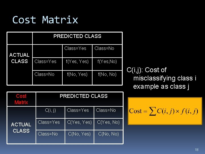
Cost Matrix PREDICTED CLASS Class=Yes ACTUAL CLASS Class=Yes Class=No Cost Matrix f(Yes, Yes) f(Yes, No) f(No, Yes) f(No, No) C(i, j): Cost of misclassifying class i example as class j PREDICTED CLASS C(i, j) ACTUAL CLASS Class=No Class=Yes C(Yes, Yes) C(Yes, No) Class=No C(No, Yes) C(No, No) 25

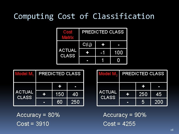
Computing Cost of Classification Cost Matrix PREDICTED CLASS ACTUAL CLASS Model M 1 ACTUAL CLASS PREDICTED CLASS + - + 150 40 - 60 250 Accuracy = 80% Cost = 3910 C(i, j) + -1 100 - 1 0 Model M 2 ACTUAL CLASS PREDICTED CLASS + - + 250 45 - 5 200 Accuracy = 90% Cost = 4255 26

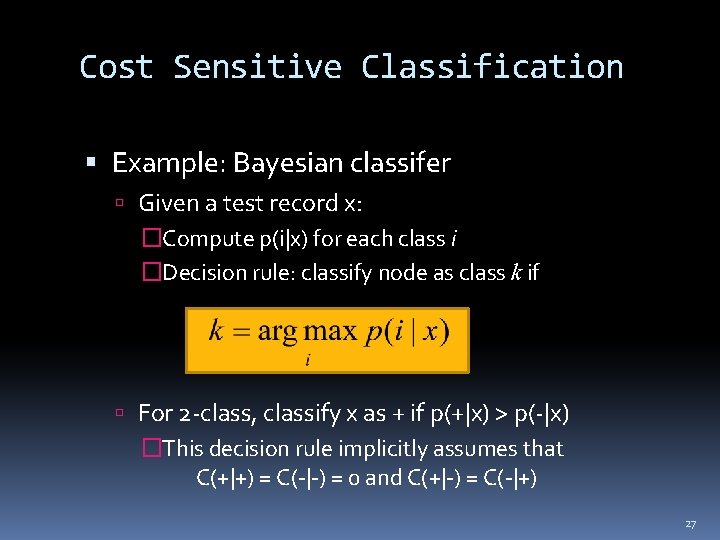
Cost Sensitive Classification Example: Bayesian classifer Given a test record x: �Compute p(i|x) for each class i �Decision rule: classify node as class k if For 2 -class, classify x as + if p(+|x) > p(-|x) �This decision rule implicitly assumes that C(+|+) = C(-|-) = 0 and C(+|-) = C(-|+) 27

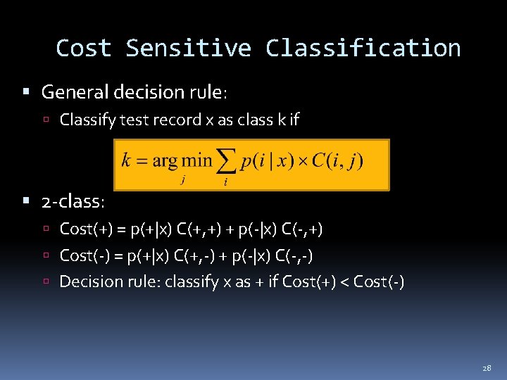
Cost Sensitive Classification General decision rule: Classify test record x as class k if 2 -class: Cost(+) = p(+|x) C(+, +) + p(-|x) C(-, +) Cost(-) = p(+|x) C(+, -) + p(-|x) C(-, -) Decision rule: classify x as + if Cost(+) < Cost(-) 28

Sampling-based Approaches Modify the distribution of training data so rare class is well-represented in training set Undersample the majority class Oversample the rare class Can try something smarter like SMOTE �SMOTE=Synthetic Minority Oversampling Technique �Generate new minority examples near other ones Advantages and disadvantages Undersampling means throwing away data (bad) Oversampling w/o SMOTE means duplicating examples that can lead to overfitting 29

DISCUSSION OF MINING WITH RARITY: A UNIFYING FRAMEWORK 30

Mining with Rarity: Unifying Framework This paper discusses: What is rarity? Why does rarity make learning difficult? How can rarity be addressed? 31

What is Rarity? Rare classes Absolute Rarity �Number of examples belonging to rare class is small and this makes it difficult to learn well Relative Rarity �Number of examples in rare class(es) is much smaller than in the common class(es). The relative difference causes problems Rare cases Within a class there may be rare cases, which correspond to sub-concepts. �For example, in medical diagnosis, there may be a class associated with “disease” and rare cases correspond to a specific rate disease. 32

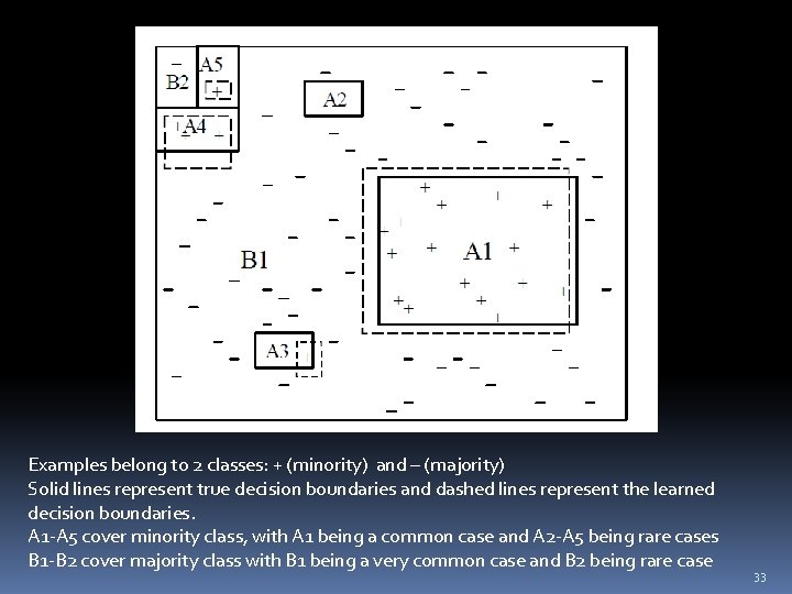
Examples belong to 2 classes: + (minority) and – (majority) Solid lines represent true decision boundaries and dashed lines represent the learned decision boundaries. A 1 -A 5 cover minority class, with A 1 being a common case and A 2 -A 5 being rare cases B 1 -B 2 cover majority class with B 1 being a very common case and B 2 being rare case 33

Why Does Rarity Make Learning Difficult? Improper evaluation metrics (e. g. , accuracy) Lack of data: absolute rarity See next slide Relative rarity: class imbalance Learners biased toward more common class Data Fragmentation Rare cases/classes affected more Inappropriate Inductive Bias Most classifiers use maximum generality bias Noise See second slide 34

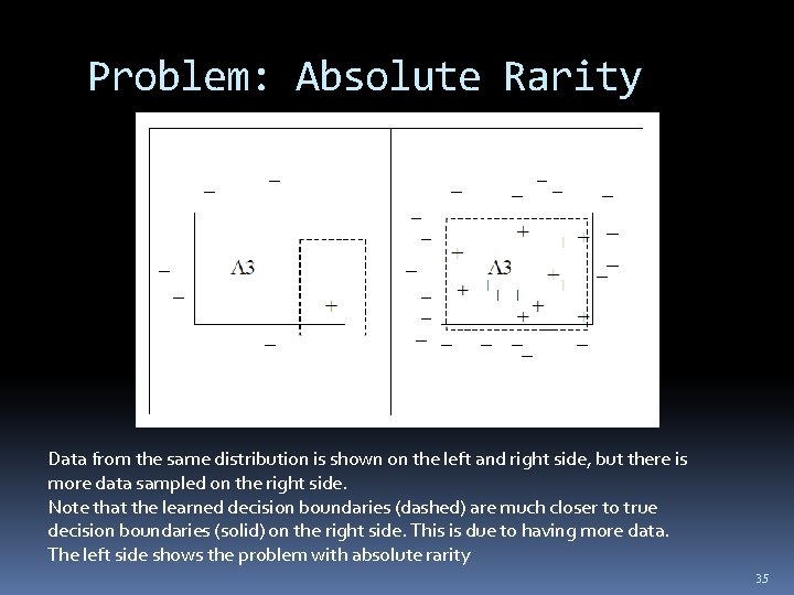
Problem: Absolute Rarity Data from the same distribution is shown on the left and right side, but there is more data sampled on the right side. Note that the learned decision boundaries (dashed) are much closer to true decision boundaries (solid) on the right side. This is due to having more data. The left side shows the problem with absolute rarity 35

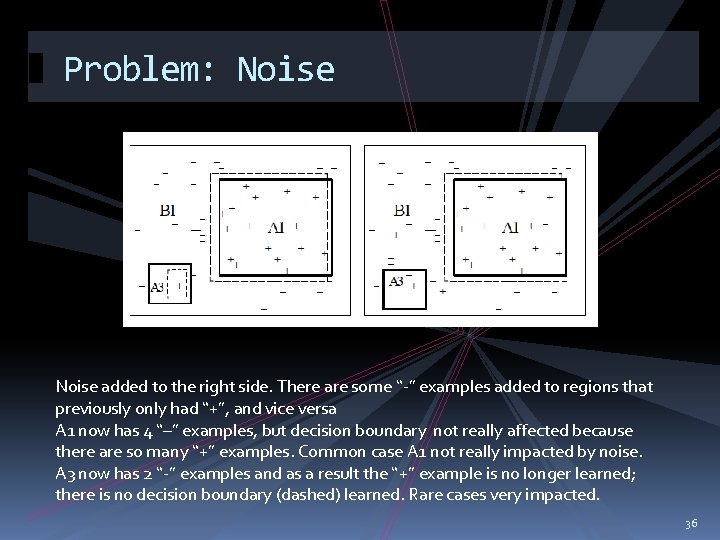
Problem: Noise added to the right side. There are some “-” examples added to regions that previously only had “+”, and vice versa A 1 now has 4 “–” examples, but decision boundary not really affected because there are so many “+” examples. Common case A 1 not really impacted by noise. A 3 now has 2 “-” examples and as a result the “+” example is no longer learned; there is no decision boundary (dashed) learned. Rare cases very impacted. 36

Methods for Addressing Rarity Use more appropriate evaluation metrics Like AUC and F 1 -measure Non-greedy search techniques More robust search methods (genetic algorithms) can identify subtle interactions between many features Use more appropriate inductive bias Knowledge/Human Interaction Human can insert domain knowledge by using good features 37

Methods for Addressing Rarity Learn only the rare class Some methods, like Ripper, use examples from all classes but can learns the rare class (Ripper uses default rule for majority class) One-class learning/recognition-based methods �Learns using data from only one class, in this case the minority class �This method is very different from methods that learn to distinguish between classes �Example: gait biometrics using sensor data. Given a sample of data from person X, assume that if new data is close to X (within a threshold) then it is from X. 38

Methods for Addressing Rarity Cost-sensitive learning If we know the actual costs for different types of errors, we can use cost-sensitive learning, which will tend to favor the minority class (usually has more costly errors) Sampling This is a very common and well studied method (see next slide) 39

Sampling Can handle class imbalance by eliminating or reducing it Oversample minority class (duplicate examples) Undersample minority class (discard examples) Do a bit of both Instead of random over/under-sampling, create new minority class examples �SMOTE: Synthetic Minority Oversampling Technique �Creates new minority examples between existing ones 40

Some Final Points In other research, I showed that examples belonging to rare class almost always have higher error rate I also showed that small disjuncts have higher error rate than large disjuncts Small disjunct are rules/leaf nodes that cover few examples There is no really good way to handle the class imbalance problem, especially if absolute rarity Ideally get more data/more minority examples 41