Data Mining Association Analysis Introduction to Data Mining

Data Mining Association Analysis Introduction to Data Mining by Tan, Steinbach, Kumar © Tan, Steinbach, Kumar Introduction to Data Mining 4/18/2004 1

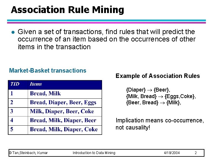
Association Rule Mining l Given a set of transactions, find rules that will predict the occurrence of an item based on the occurrences of other items in the transaction Market-Basket transactions Example of Association Rules {Diaper} {Beer}, {Milk, Bread} {Eggs, Coke}, {Beer, Bread} {Milk}, Implication means co-occurrence, not causality! © Tan, Steinbach, Kumar Introduction to Data Mining 4/18/2004 2

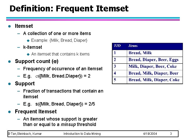
Definition: Frequent Itemset l Itemset – A collection of one or more items u Example: {Milk, Bread, Diaper} – k-itemset u l An itemset that contains k items Support count ( ) – Frequency of occurrence of an itemset – E. g. ({Milk, Bread, Diaper}) = 2 l Support – Fraction of transactions that contain an itemset – E. g. s({Milk, Bread, Diaper}) = 2/5 l Frequent Itemset – An itemset whose support is greater than or equal to a minsup threshold © Tan, Steinbach, Kumar Introduction to Data Mining 4/18/2004 3

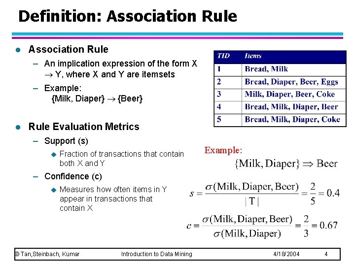
Definition: Association Rule l Association Rule – An implication expression of the form X Y, where X and Y are itemsets – Example: {Milk, Diaper} {Beer} l Rule Evaluation Metrics – Support (s) u Fraction of transactions that contain both X and Y Example: – Confidence (c) u Measures how often items in Y appear in transactions that contain X © Tan, Steinbach, Kumar Introduction to Data Mining 4/18/2004 4

Association Rule Mining Task l Given a set of transactions T, the goal of association rule mining is to find all rules having – support ≥ minsup threshold – confidence ≥ minconf threshold l Brute-force approach: – List all possible association rules – Compute the support and confidence for each rule – Prune rules that fail the minsup and minconf thresholds Computationally prohibitive! © Tan, Steinbach, Kumar Introduction to Data Mining 4/18/2004 5

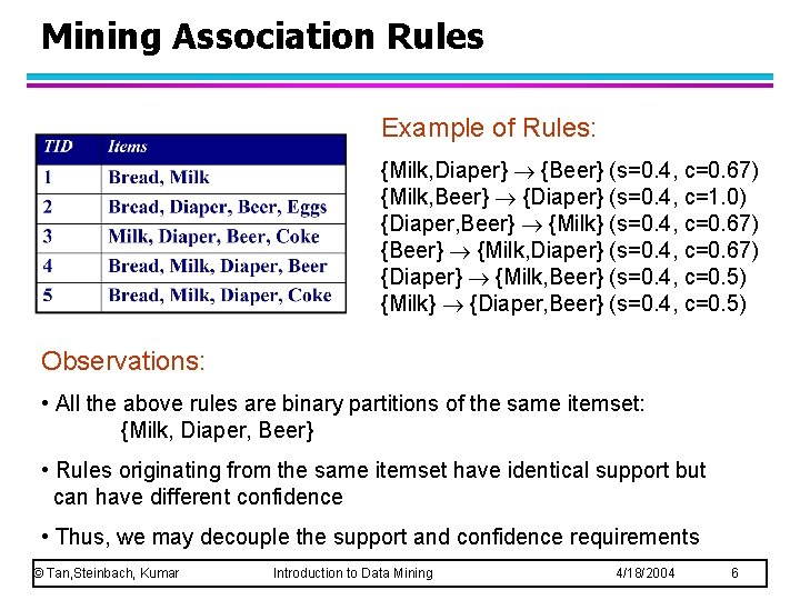
Mining Association Rules Example of Rules: {Milk, Diaper} {Beer} (s=0. 4, c=0. 67) {Milk, Beer} {Diaper} (s=0. 4, c=1. 0) {Diaper, Beer} {Milk} (s=0. 4, c=0. 67) {Beer} {Milk, Diaper} (s=0. 4, c=0. 67) {Diaper} {Milk, Beer} (s=0. 4, c=0. 5) {Milk} {Diaper, Beer} (s=0. 4, c=0. 5) Observations: • All the above rules are binary partitions of the same itemset: {Milk, Diaper, Beer} • Rules originating from the same itemset have identical support but can have different confidence • Thus, we may decouple the support and confidence requirements © Tan, Steinbach, Kumar Introduction to Data Mining 4/18/2004 6

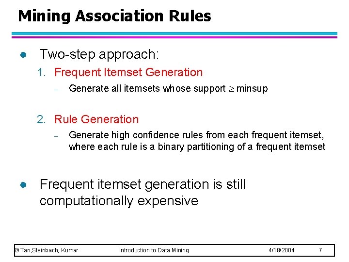
Mining Association Rules l Two-step approach: 1. Frequent Itemset Generation – Generate all itemsets whose support minsup 2. Rule Generation – l Generate high confidence rules from each frequent itemset, where each rule is a binary partitioning of a frequent itemset Frequent itemset generation is still computationally expensive © Tan, Steinbach, Kumar Introduction to Data Mining 4/18/2004 7

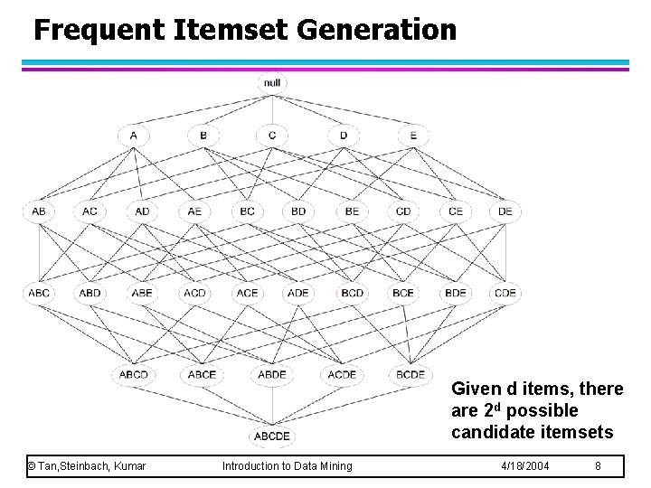
Frequent Itemset Generation Given d items, there are 2 d possible candidate itemsets © Tan, Steinbach, Kumar Introduction to Data Mining 4/18/2004 8

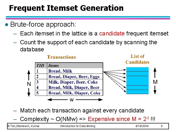
Frequent Itemset Generation l Brute-force approach: – Each itemset in the lattice is a candidate frequent itemset – Count the support of each candidate by scanning the database – Match each transaction against every candidate – Complexity ~ O(NMw) => Expensive since M = 2 d !!! © Tan, Steinbach, Kumar Introduction to Data Mining 4/18/2004 9

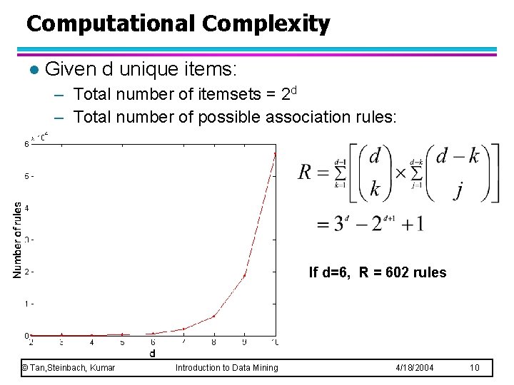
Computational Complexity l Given d unique items: – Total number of itemsets = 2 d – Total number of possible association rules: If d=6, R = 602 rules © Tan, Steinbach, Kumar Introduction to Data Mining 4/18/2004 10

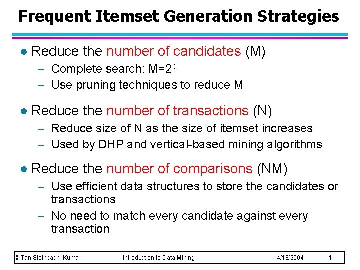
Frequent Itemset Generation Strategies l Reduce the number of candidates (M) – Complete search: M=2 d – Use pruning techniques to reduce M l Reduce the number of transactions (N) – Reduce size of N as the size of itemset increases – Used by DHP and vertical-based mining algorithms l Reduce the number of comparisons (NM) – Use efficient data structures to store the candidates or transactions – No need to match every candidate against every transaction © Tan, Steinbach, Kumar Introduction to Data Mining 4/18/2004 11

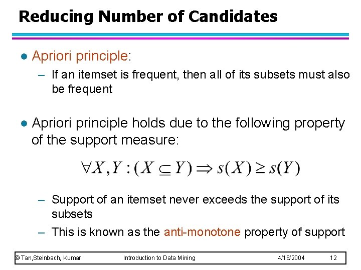
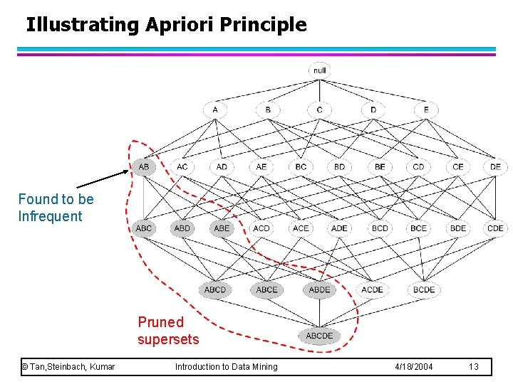
Reducing Number of Candidates l Apriori principle: – If an itemset is frequent, then all of its subsets must also be frequent l Apriori principle holds due to the following property of the support measure: – Support of an itemset never exceeds the support of its subsets – This is known as the anti-monotone property of support © Tan, Steinbach, Kumar Introduction to Data Mining 4/18/2004 12

Illustrating Apriori Principle Found to be Infrequent Pruned supersets © Tan, Steinbach, Kumar Introduction to Data Mining 4/18/2004 13

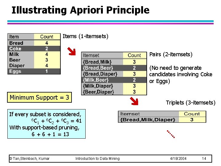
Illustrating Apriori Principle Items (1 -itemsets) Pairs (2 -itemsets) (No need to generate candidates involving Coke or Eggs) Minimum Support = 3 Triplets (3 -itemsets) If every subset is considered, 6 C + 6 C = 41 1 2 3 With support-based pruning, 6 + 1 = 13 © Tan, Steinbach, Kumar Introduction to Data Mining 4/18/2004 14

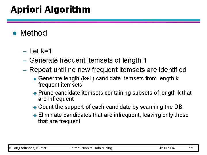
Apriori Algorithm l Method: – Let k=1 – Generate frequent itemsets of length 1 – Repeat until no new frequent itemsets are identified u Generate length (k+1) candidate itemsets from length k frequent itemsets u Prune candidate itemsets containing subsets of length k that are infrequent u Count the support of each candidate by scanning the DB u Eliminate candidates that are infrequent, leaving only those that are frequent © Tan, Steinbach, Kumar Introduction to Data Mining 4/18/2004 15

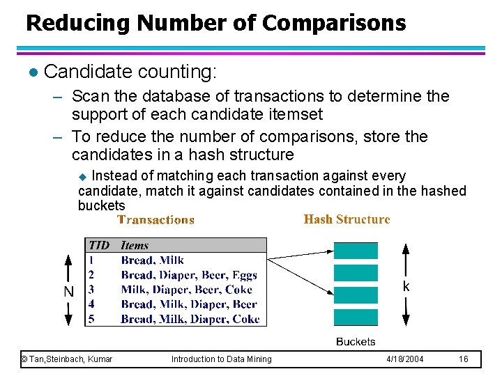
Reducing Number of Comparisons l Candidate counting: – Scan the database of transactions to determine the support of each candidate itemset – To reduce the number of comparisons, store the candidates in a hash structure Instead of matching each transaction against every candidate, match it against candidates contained in the hashed buckets u © Tan, Steinbach, Kumar Introduction to Data Mining 4/18/2004 16

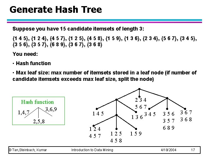
Generate Hash Tree Suppose you have 15 candidate itemsets of length 3: {1 4 5}, {1 2 4}, {4 5 7}, {1 2 5}, {4 5 8}, {1 5 9}, {1 3 6}, {2 3 4}, {5 6 7}, {3 4 5}, {3 5 6}, {3 5 7}, {6 8 9}, {3 6 7}, {3 6 8} You need: • Hash function • Max leaf size: max number of itemsets stored in a leaf node (if number of candidate itemsets exceeds max leaf size, split the node) Hash function 3, 6, 9 1, 4, 7 234 567 345 136 145 2, 5, 8 124 457 © Tan, Steinbach, Kumar 125 458 Introduction to Data Mining 159 356 357 689 4/18/2004 367 368 17

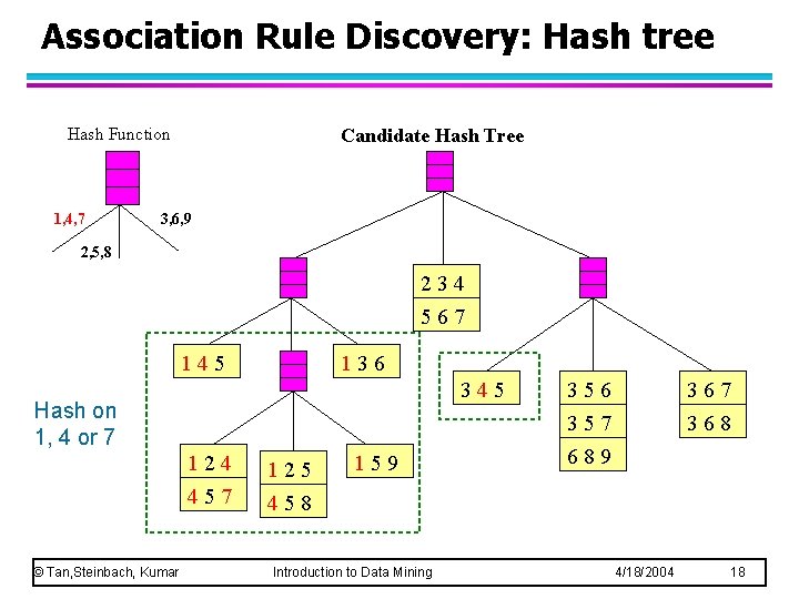
Association Rule Discovery: Hash tree Hash Function 1, 4, 7 Candidate Hash Tree 3, 6, 9 2, 5, 8 234 567 145 136 345 Hash on 1, 4 or 7 © Tan, Steinbach, Kumar 124 125 457 458 159 Introduction to Data Mining 356 367 368 357 689 4/18/2004 18

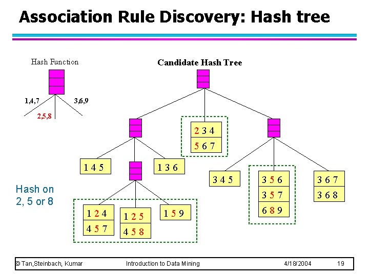
Association Rule Discovery: Hash tree Hash Function 1, 4, 7 Candidate Hash Tree 3, 6, 9 2, 5, 8 234 567 145 136 345 Hash on 2, 5 or 8 © Tan, Steinbach, Kumar 124 125 457 458 159 Introduction to Data Mining 356 367 368 357 689 4/18/2004 19

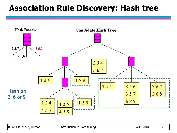
Association Rule Discovery: Hash tree Hash Function 1, 4, 7 Candidate Hash Tree 3, 6, 9 2, 5, 8 234 567 145 136 345 Hash on 3, 6 or 9 © Tan, Steinbach, Kumar 124 125 457 458 159 Introduction to Data Mining 356 367 368 357 689 4/18/2004 20

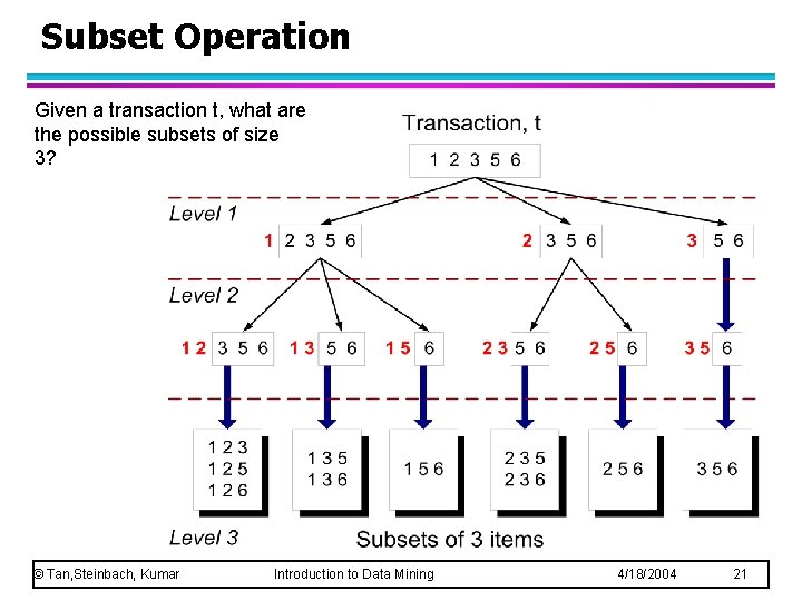
Subset Operation Given a transaction t, what are the possible subsets of size 3? © Tan, Steinbach, Kumar Introduction to Data Mining 4/18/2004 21

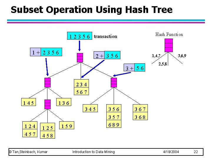
Subset Operation Using Hash Tree Hash Function 1 2 3 5 6 transaction 1+ 2356 2+ 356 1, 4, 7 3+ 56 3, 6, 9 2, 5, 8 234 567 145 136 345 124 457 125 458 © Tan, Steinbach, Kumar 159 356 357 689 Introduction to Data Mining 367 368 4/18/2004 22

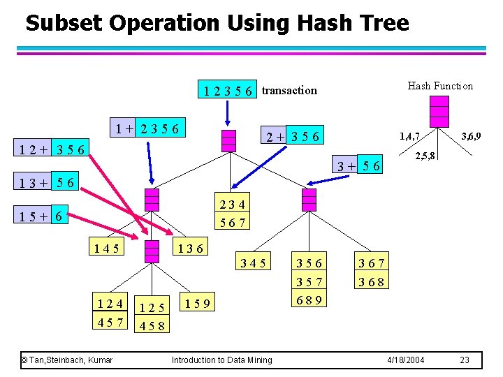
Subset Operation Using Hash Tree Hash Function 1 2 3 5 6 transaction 1+ 2356 2+ 356 1, 4, 7 3+ 56 3, 6, 9 2, 5, 8 13+ 56 234 567 15+ 6 145 136 345 124 457 © Tan, Steinbach, Kumar 125 458 159 Introduction to Data Mining 356 357 689 367 368 4/18/2004 23

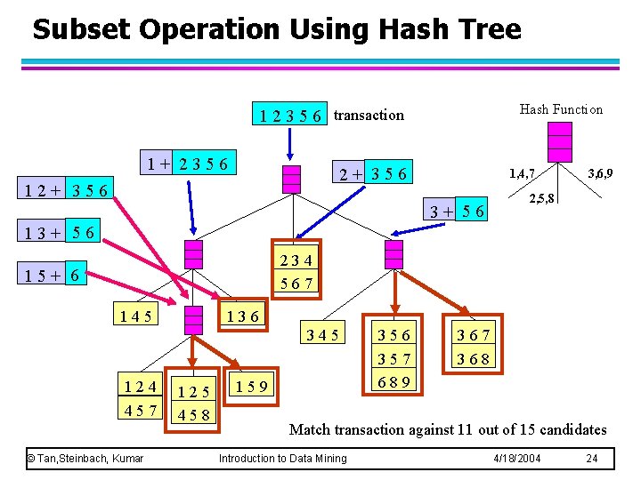
Subset Operation Using Hash Tree Hash Function 1 2 3 5 6 transaction 1+ 2356 2+ 356 1, 4, 7 3+ 56 3, 6, 9 2, 5, 8 13+ 56 234 567 15+ 6 145 136 345 124 457 © Tan, Steinbach, Kumar 125 458 159 356 357 689 367 368 Match transaction against 11 out of 15 candidates Introduction to Data Mining 4/18/2004 24

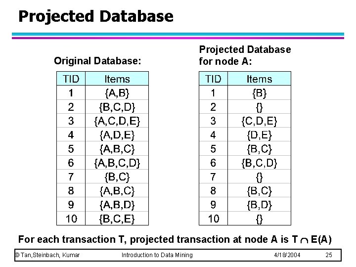
Projected Database Original Database: Projected Database for node A: For each transaction T, projected transaction at node A is T E(A) © Tan, Steinbach, Kumar Introduction to Data Mining 4/18/2004 25

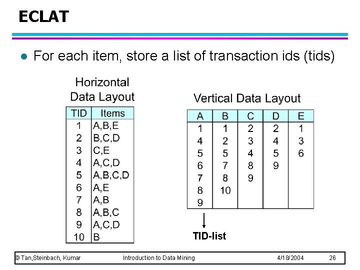
ECLAT l For each item, store a list of transaction ids (tids) TID-list © Tan, Steinbach, Kumar Introduction to Data Mining 4/18/2004 26

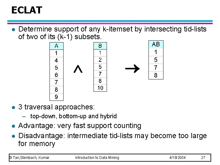
ECLAT l Determine support of any k-itemset by intersecting tid-lists of two of its (k-1) subsets. l 3 traversal approaches: – top-down, bottom-up and hybrid l l Advantage: very fast support counting Disadvantage: intermediate tid-lists may become too large for memory © Tan, Steinbach, Kumar Introduction to Data Mining 4/18/2004 27

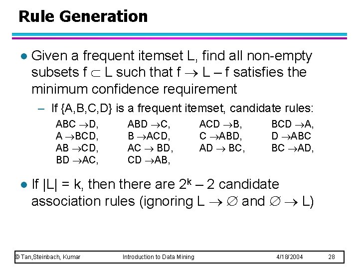
Rule Generation l Given a frequent itemset L, find all non-empty subsets f L such that f L – f satisfies the minimum confidence requirement – If {A, B, C, D} is a frequent itemset, candidate rules: ABC D, A BCD, AB CD, BD AC, l ABD C, B ACD, AC BD, CD AB, ACD B, C ABD, AD BC, BCD A, D ABC BC AD, If |L| = k, then there are 2 k – 2 candidate association rules (ignoring L and L) © Tan, Steinbach, Kumar Introduction to Data Mining 4/18/2004 28

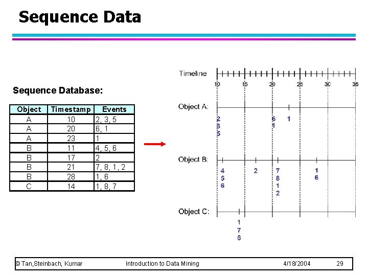
Sequence Database: Object A A A B B C Timestamp 10 20 23 11 17 21 28 14 © Tan, Steinbach, Kumar Events 2, 3, 5 6, 1 1 4, 5, 6 2 7, 8, 1, 2 1, 6 1, 8, 7 Introduction to Data Mining 4/18/2004 29

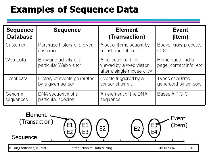
Examples of Sequence Database Sequence Element (Transaction) Event (Item) Customer Purchase history of a given customer A set of items bought by a customer at time t Books, diary products, CDs, etc Web Data Browsing activity of a particular Web visitor A collection of files viewed by a Web visitor after a single mouse click Home page, index page, contact info, etc Event data History of events generated by a given sensor Events triggered by a sensor at time t Types of alarms generated by sensors Genome sequences DNA sequence of a particular species An element of the DNA sequence Bases A, T, G, C Element (Transaction) Sequence © Tan, Steinbach, Kumar E 1 E 2 E 1 E 3 E 2 Introduction to Data Mining E 2 E 3 E 4 Event (Item) 4/18/2004 30

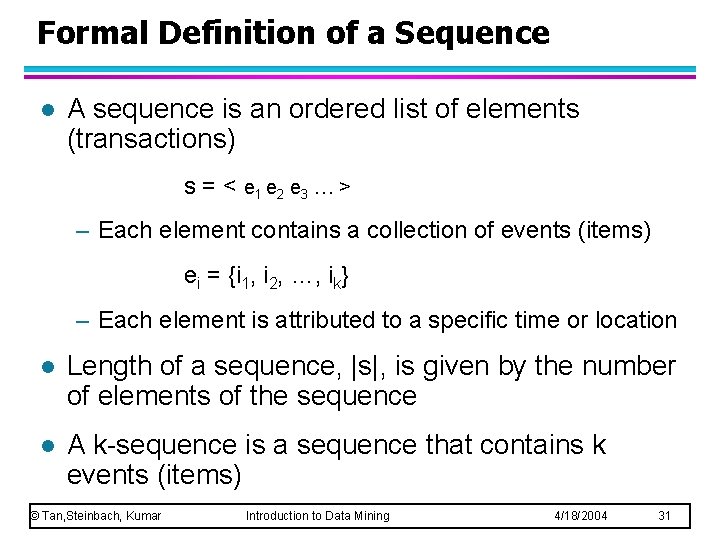
Formal Definition of a Sequence l A sequence is an ordered list of elements (transactions) s = < e 1 e 2 e 3 … > – Each element contains a collection of events (items) ei = {i 1, i 2, …, ik} – Each element is attributed to a specific time or location l Length of a sequence, |s|, is given by the number of elements of the sequence l A k-sequence is a sequence that contains k events (items) © Tan, Steinbach, Kumar Introduction to Data Mining 4/18/2004 31

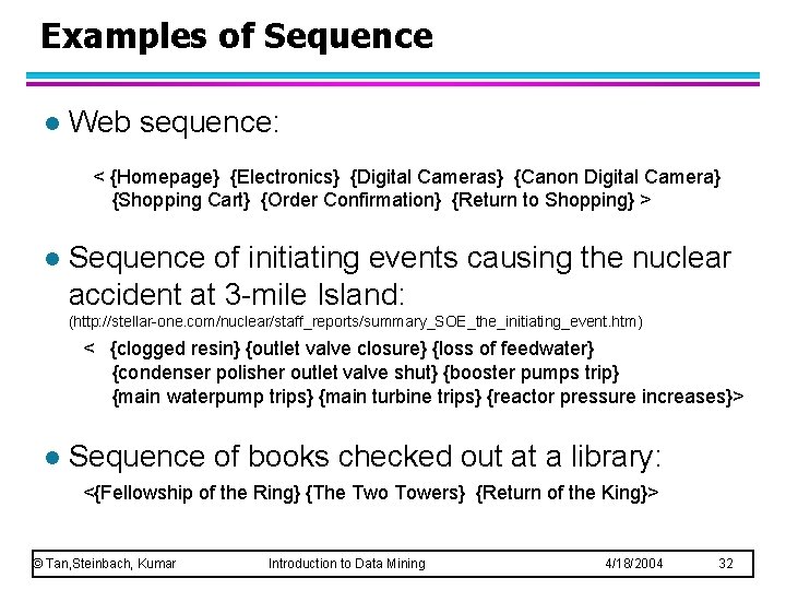
Examples of Sequence l Web sequence: < {Homepage} {Electronics} {Digital Cameras} {Canon Digital Camera} {Shopping Cart} {Order Confirmation} {Return to Shopping} > l Sequence of initiating events causing the nuclear accident at 3 -mile Island: (http: //stellar-one. com/nuclear/staff_reports/summary_SOE_the_initiating_event. htm) < {clogged resin} {outlet valve closure} {loss of feedwater} {condenser polisher outlet valve shut} {booster pumps trip} {main waterpump trips} {main turbine trips} {reactor pressure increases}> l Sequence of books checked out at a library: <{Fellowship of the Ring} {The Two Towers} {Return of the King}> © Tan, Steinbach, Kumar Introduction to Data Mining 4/18/2004 32

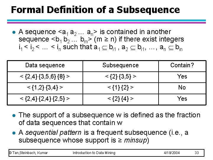
Formal Definition of a Subsequence l l l A sequence <a 1 a 2 … an> is contained in another sequence <b 1 b 2 … bm> (m ≥ n) if there exist integers i 1 < i 2 < … < in such that a 1 bi 1 , a 2 bi 1, …, an bin Data sequence Subsequence Contain? < {2, 4} {3, 5, 6} {8} > < {2} {3, 5} > Yes < {1, 2} {3, 4} > < {1} {2} > No < {2, 4} {2, 5} > < {2} {4} > Yes The support of a subsequence w is defined as the fraction of data sequences that contain w A sequential pattern is a frequent subsequence (i. e. , a subsequence whose support is ≥ minsup) © Tan, Steinbach, Kumar Introduction to Data Mining 4/18/2004 33

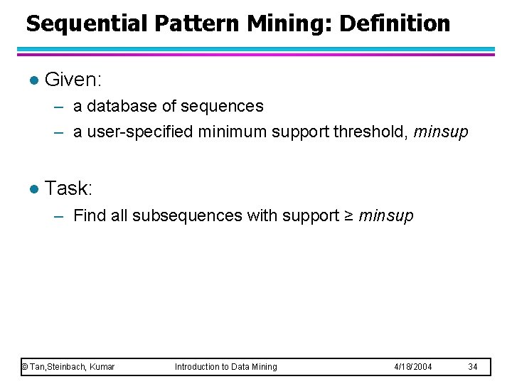
Sequential Pattern Mining: Definition l Given: – a database of sequences – a user-specified minimum support threshold, minsup l Task: – Find all subsequences with support ≥ minsup © Tan, Steinbach, Kumar Introduction to Data Mining 4/18/2004 34

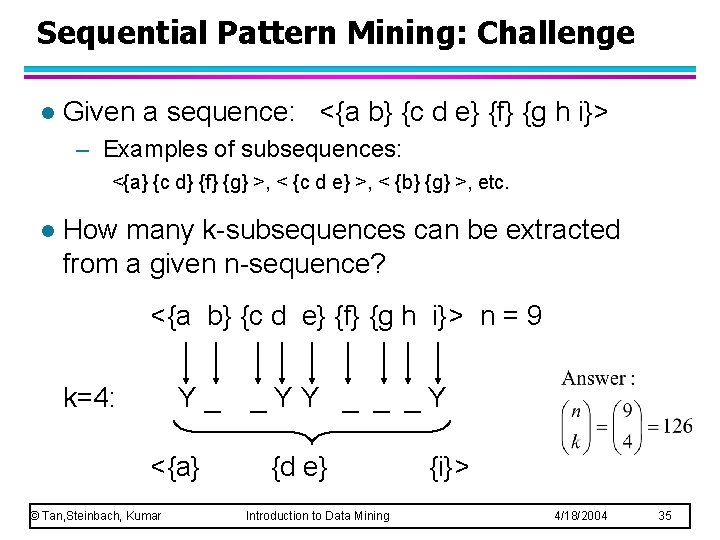
Sequential Pattern Mining: Challenge l Given a sequence: <{a b} {c d e} {f} {g h i}> – Examples of subsequences: <{a} {c d} {f} {g} >, < {c d e} >, < {b} {g} >, etc. l How many k-subsequences can be extracted from a given n-sequence? <{a b} {c d e} {f} {g h i}> n = 9 k=4: Y_ <{a} © Tan, Steinbach, Kumar _YY _ _ _Y {d e} Introduction to Data Mining {i}> 4/18/2004 35

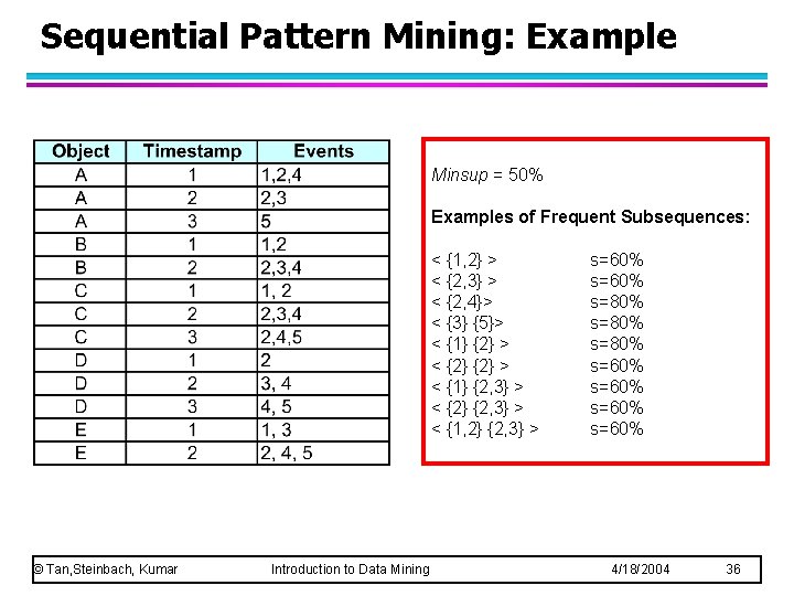
Sequential Pattern Mining: Example Minsup = 50% Examples of Frequent Subsequences: < {1, 2} > < {2, 3} > < {2, 4}> < {3} {5}> < {1} {2} > < {1} {2, 3} > < {2} {2, 3} > < {1, 2} {2, 3} > © Tan, Steinbach, Kumar Introduction to Data Mining s=60% s=80% s=60% 4/18/2004 36

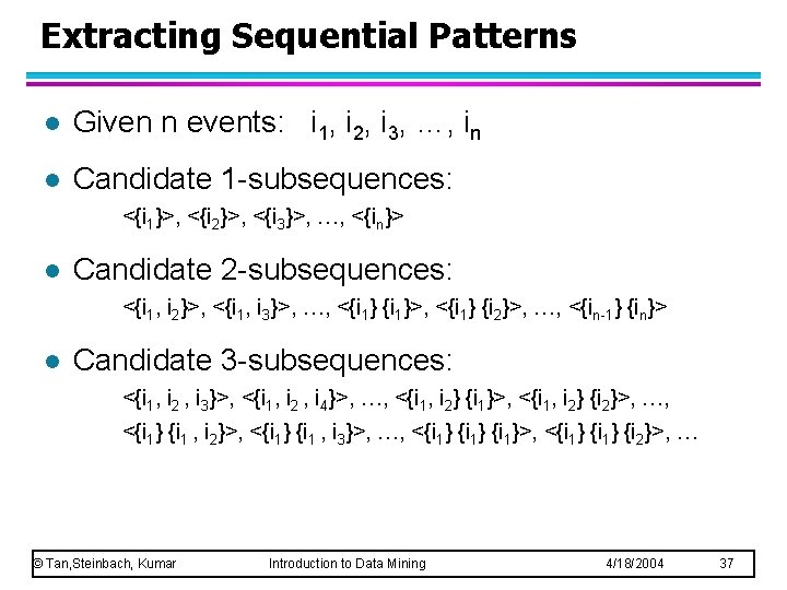
Extracting Sequential Patterns l Given n events: i 1, i 2, i 3, …, in l Candidate 1 -subsequences: <{i 1}>, <{i 2}>, <{i 3}>, …, <{in}> l Candidate 2 -subsequences: <{i 1, i 2}>, <{i 1, i 3}>, …, <{i 1}>, <{i 1} {i 2}>, …, <{in-1} {in}> l Candidate 3 -subsequences: <{i 1, i 2 , i 3}>, <{i 1, i 2 , i 4}>, …, <{i 1, i 2} {i 1}>, <{i 1, i 2} {i 2}>, …, <{i 1} {i 1 , i 2}>, <{i 1} {i 1 , i 3}>, …, <{i 1}>, <{i 1} {i 2}>, … © Tan, Steinbach, Kumar Introduction to Data Mining 4/18/2004 37

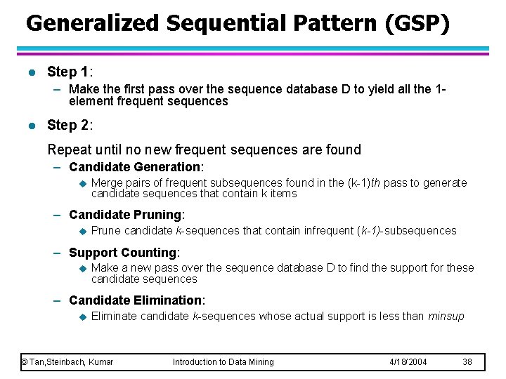
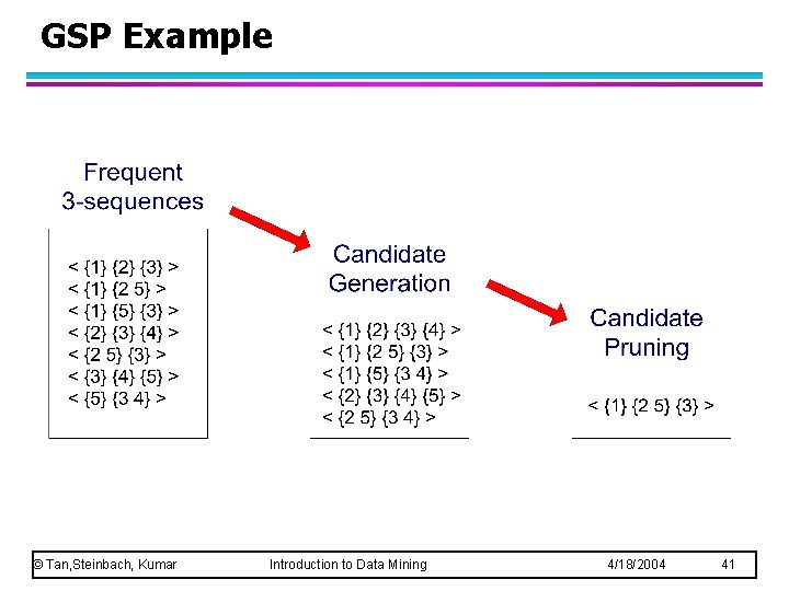
Generalized Sequential Pattern (GSP) l Step 1: – Make the first pass over the sequence database D to yield all the 1 element frequent sequences l Step 2: Repeat until no new frequent sequences are found – Candidate Generation: u Merge pairs of frequent subsequences found in the (k-1)th pass to generate candidate sequences that contain k items – Candidate Pruning: u Prune candidate k-sequences that contain infrequent (k-1)-subsequences – Support Counting: u Make a new pass over the sequence database D to find the support for these candidate sequences – Candidate Elimination: u Eliminate candidate k-sequences whose actual support is less than minsup © Tan, Steinbach, Kumar Introduction to Data Mining 4/18/2004 38

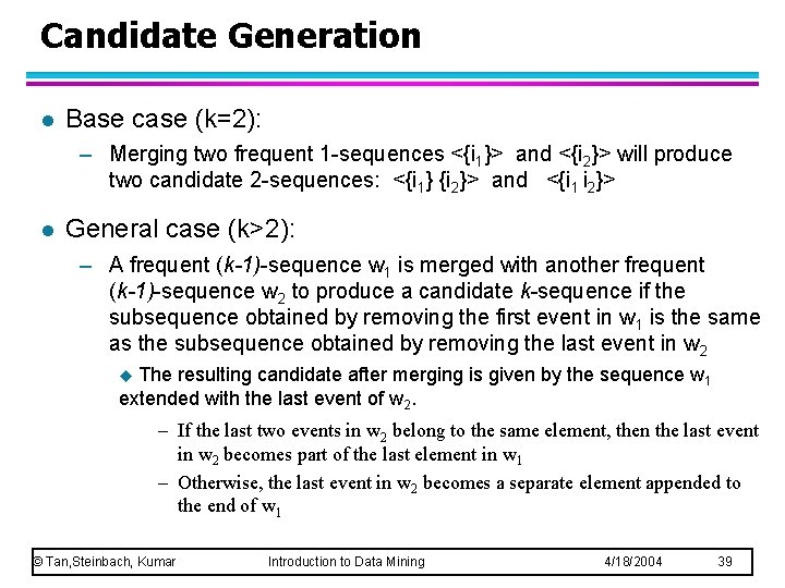
Candidate Generation l Base case (k=2): – Merging two frequent 1 -sequences <{i 1}> and <{i 2}> will produce two candidate 2 -sequences: <{i 1} {i 2}> and <{i 1 i 2}> l General case (k>2): – A frequent (k-1)-sequence w 1 is merged with another frequent (k-1)-sequence w 2 to produce a candidate k-sequence if the subsequence obtained by removing the first event in w 1 is the same as the subsequence obtained by removing the last event in w 2 The resulting candidate after merging is given by the sequence w 1 extended with the last event of w 2. u – If the last two events in w 2 belong to the same element, then the last event in w 2 becomes part of the last element in w 1 – Otherwise, the last event in w 2 becomes a separate element appended to the end of w 1 © Tan, Steinbach, Kumar Introduction to Data Mining 4/18/2004 39

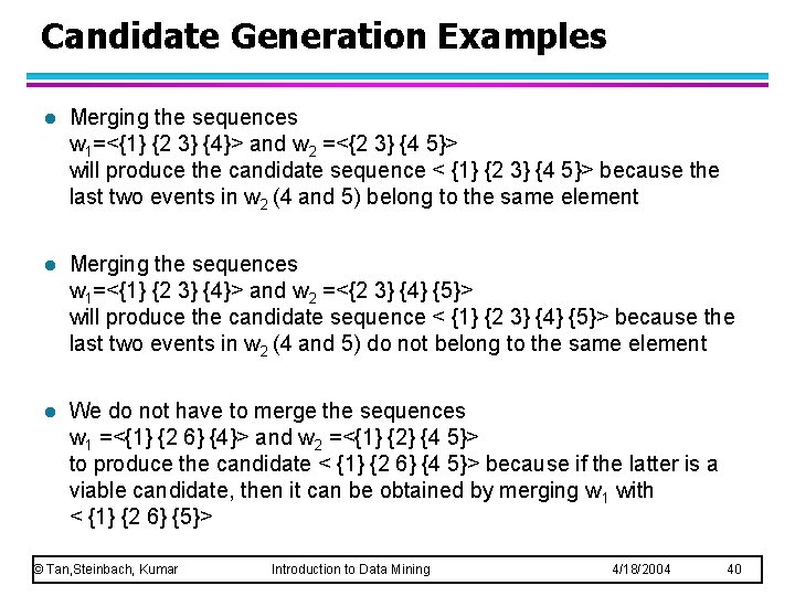
Candidate Generation Examples l Merging the sequences w 1=<{1} {2 3} {4}> and w 2 =<{2 3} {4 5}> will produce the candidate sequence < {1} {2 3} {4 5}> because the last two events in w 2 (4 and 5) belong to the same element l Merging the sequences w 1=<{1} {2 3} {4}> and w 2 =<{2 3} {4} {5}> will produce the candidate sequence < {1} {2 3} {4} {5}> because the last two events in w 2 (4 and 5) do not belong to the same element l We do not have to merge the sequences w 1 =<{1} {2 6} {4}> and w 2 =<{1} {2} {4 5}> to produce the candidate < {1} {2 6} {4 5}> because if the latter is a viable candidate, then it can be obtained by merging w 1 with < {1} {2 6} {5}> © Tan, Steinbach, Kumar Introduction to Data Mining 4/18/2004 40

GSP Example © Tan, Steinbach, Kumar Introduction to Data Mining 4/18/2004 41

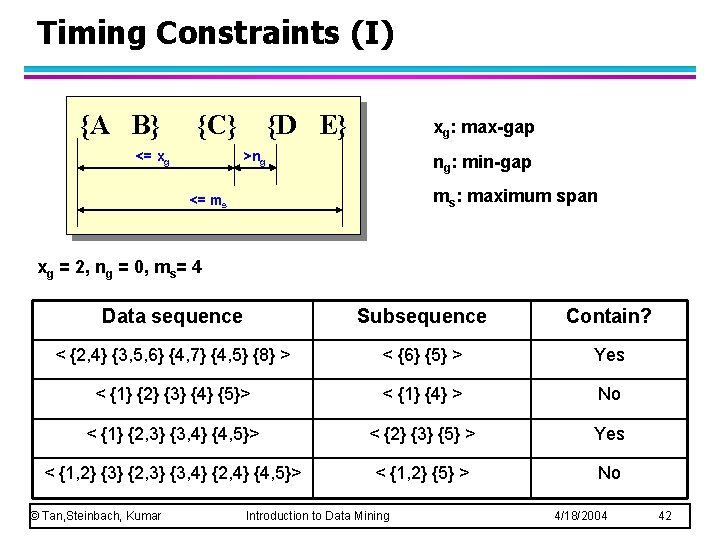
Timing Constraints (I) {A B} {C} <= xg {D E} xg: max-gap >ng ng: min-gap ms: maximum span <= ms xg = 2, ng = 0, ms= 4 Data sequence Subsequence Contain? < {2, 4} {3, 5, 6} {4, 7} {4, 5} {8} > < {6} {5} > Yes < {1} {2} {3} {4} {5}> < {1} {4} > No < {1} {2, 3} {3, 4} {4, 5}> < {2} {3} {5} > Yes < {1, 2} {3} {2, 3} {3, 4} {2, 4} {4, 5}> < {1, 2} {5} > No © Tan, Steinbach, Kumar Introduction to Data Mining 4/18/2004 42

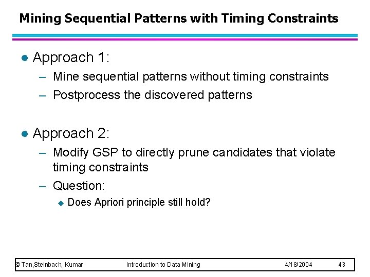
Mining Sequential Patterns with Timing Constraints l Approach 1: – Mine sequential patterns without timing constraints – Postprocess the discovered patterns l Approach 2: – Modify GSP to directly prune candidates that violate timing constraints – Question: u Does Apriori principle still hold? © Tan, Steinbach, Kumar Introduction to Data Mining 4/18/2004 43

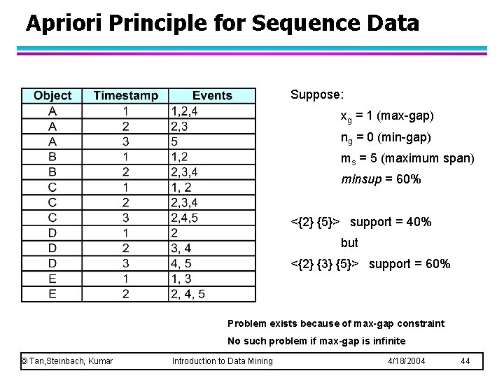
Apriori Principle for Sequence Data Suppose: xg = 1 (max-gap) ng = 0 (min-gap) ms = 5 (maximum span) minsup = 60% <{2} {5}> support = 40% but <{2} {3} {5}> support = 60% Problem exists because of max-gap constraint No such problem if max-gap is infinite © Tan, Steinbach, Kumar Introduction to Data Mining 4/18/2004 44

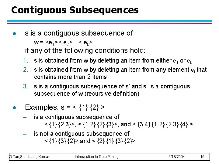
Contiguous Subsequences l s is a contiguous subsequence of w = <e 1>< e 2>…< ek> if any of the following conditions hold: 1. s is obtained from w by deleting an item from either e 1 or ek 2. s is obtained from w by deleting an item from any element ei that contains more than 2 items 3. s is a contiguous subsequence of s’ and s’ is a contiguous subsequence of w (recursive definition) l Examples: s = < {1} {2} > – is a contiguous subsequence of < {1} {2 3}>, < {1 2} {3}>, and < {3 4} {1 2} {2 3} {4} > – is not a contiguous subsequence of < {1} {3} {2}> and < {2} {1} {3} {2}> © Tan, Steinbach, Kumar Introduction to Data Mining 4/18/2004 45

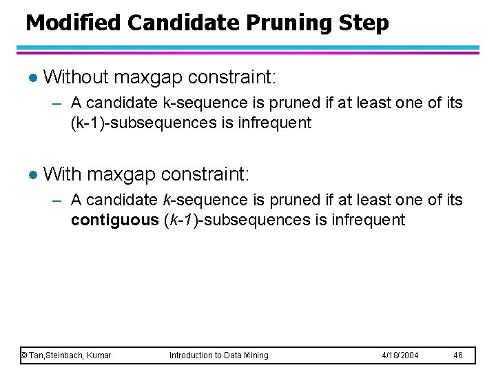
Modified Candidate Pruning Step l Without maxgap constraint: – A candidate k-sequence is pruned if at least one of its (k-1)-subsequences is infrequent l With maxgap constraint: – A candidate k-sequence is pruned if at least one of its contiguous (k-1)-subsequences is infrequent © Tan, Steinbach, Kumar Introduction to Data Mining 4/18/2004 46

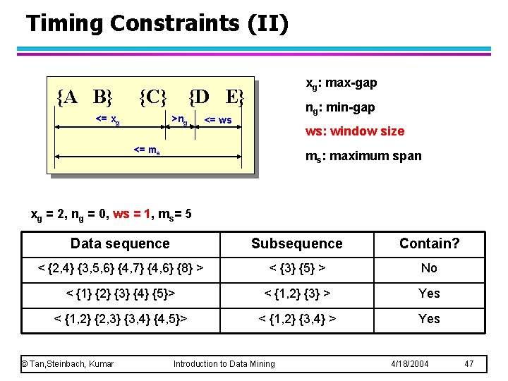
Timing Constraints (II) {A B} {C} <= xg xg: max-gap {D E} >ng ng: min-gap <= ws ws: window size <= ms ms: maximum span xg = 2, ng = 0, ws = 1, ms= 5 Data sequence Subsequence Contain? < {2, 4} {3, 5, 6} {4, 7} {4, 6} {8} > < {3} {5} > No < {1} {2} {3} {4} {5}> < {1, 2} {3} > Yes < {1, 2} {2, 3} {3, 4} {4, 5}> < {1, 2} {3, 4} > Yes © Tan, Steinbach, Kumar Introduction to Data Mining 4/18/2004 47

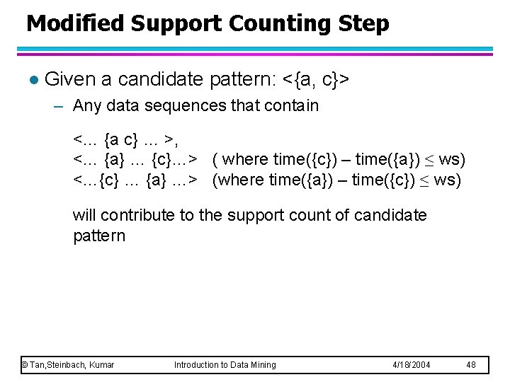
Modified Support Counting Step l Given a candidate pattern: <{a, c}> – Any data sequences that contain <… {a c} … >, <… {a} … {c}…> ( where time({c}) – time({a}) ≤ ws) <…{c} … {a} …> (where time({a}) – time({c}) ≤ ws) will contribute to the support count of candidate pattern © Tan, Steinbach, Kumar Introduction to Data Mining 4/18/2004 48

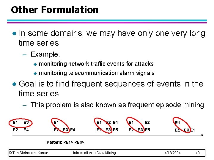
Other Formulation l In some domains, we may have only one very long time series – Example: l u monitoring network traffic events for attacks u monitoring telecommunication alarm signals Goal is to find frequent sequences of events in the time series – This problem is also known as frequent episode mining E 1 E 3 E 1 E 2 E 4 E 2 E 3 E 5 E 1 E 2 E 3 E 1 Pattern: <E 1> <E 3> © Tan, Steinbach, Kumar Introduction to Data Mining 4/18/2004 49

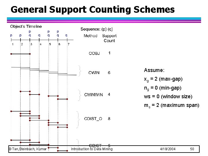
General Support Counting Schemes Assume: xg = 2 (max-gap) ng = 0 (min-gap) ws = 0 (window size) ms = 2 (maximum span) © Tan, Steinbach, Kumar Introduction to Data Mining 4/18/2004 50

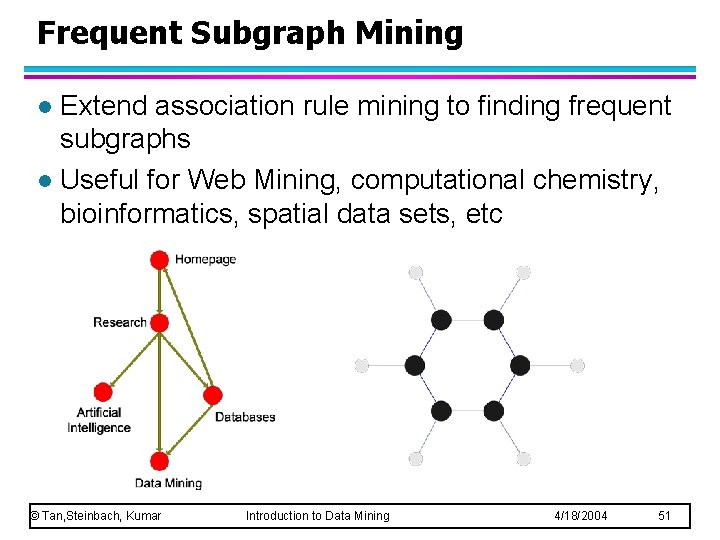
Frequent Subgraph Mining Extend association rule mining to finding frequent subgraphs l Useful for Web Mining, computational chemistry, bioinformatics, spatial data sets, etc l © Tan, Steinbach, Kumar Introduction to Data Mining 4/18/2004 51

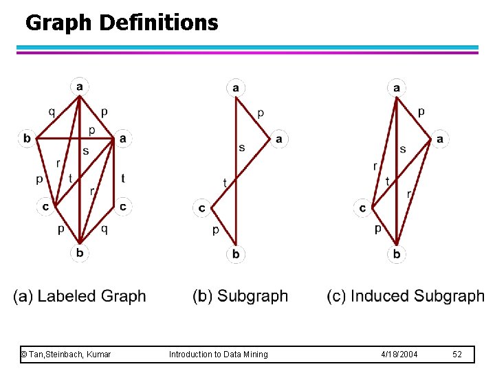
Graph Definitions © Tan, Steinbach, Kumar Introduction to Data Mining 4/18/2004 52

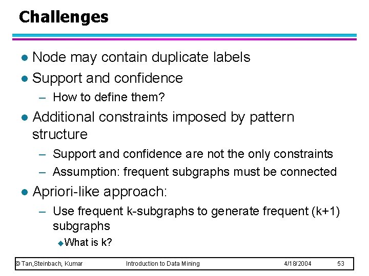
Challenges Node may contain duplicate labels l Support and confidence l – How to define them? l Additional constraints imposed by pattern structure – Support and confidence are not the only constraints – Assumption: frequent subgraphs must be connected l Apriori-like approach: – Use frequent k-subgraphs to generate frequent (k+1) subgraphs u. What © Tan, Steinbach, Kumar is k? Introduction to Data Mining 4/18/2004 53

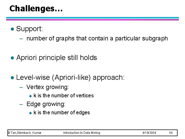
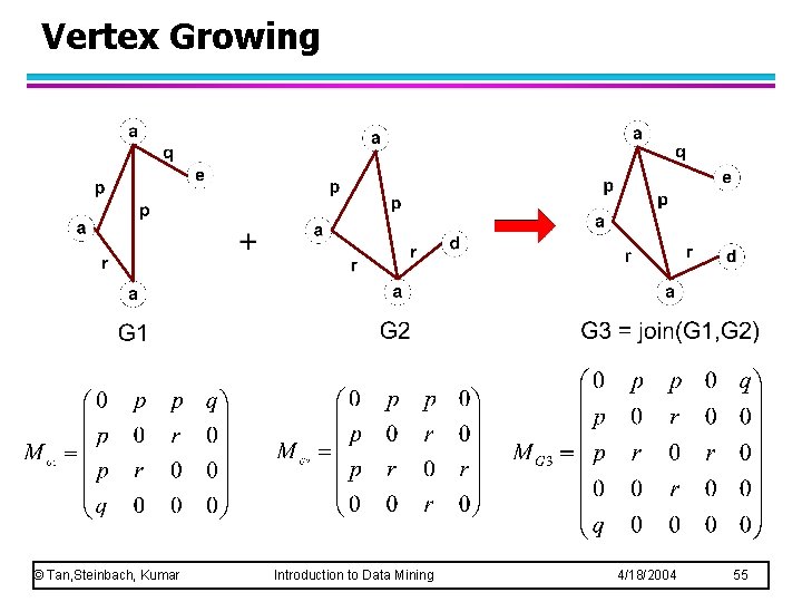
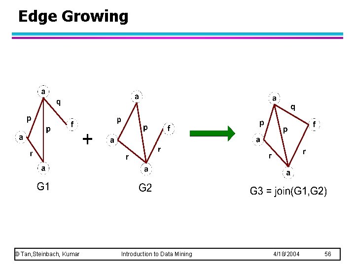
Challenges… l Support: – number of graphs that contain a particular subgraph l Apriori principle still holds l Level-wise (Apriori-like) approach: – Vertex growing: u k is the number of vertices – Edge growing: u k is the number of edges © Tan, Steinbach, Kumar Introduction to Data Mining 4/18/2004 54

Vertex Growing © Tan, Steinbach, Kumar Introduction to Data Mining 4/18/2004 55

Edge Growing © Tan, Steinbach, Kumar Introduction to Data Mining 4/18/2004 56

Apriori-like Algorithm Find frequent 1 -subgraphs l Repeat l – Candidate generation u Use frequent (k-1)-subgraphs to generate candidate k-subgraph – Candidate pruning Prune candidate subgraphs that contain infrequent (k-1)-subgraphs u – Support counting u Count the support of each remaining candidate – Eliminate candidate k-subgraphs that are infrequent In practice, it is not as easy. There are many other issues © Tan, Steinbach, Kumar Introduction to Data Mining 4/18/2004 57

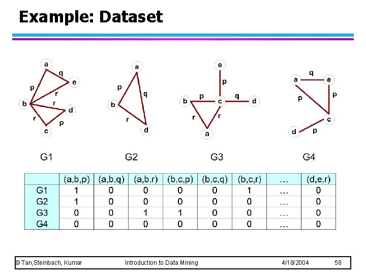
Example: Dataset © Tan, Steinbach, Kumar Introduction to Data Mining 4/18/2004 58

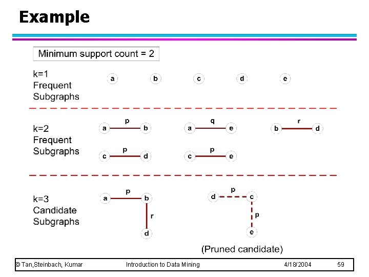
Example © Tan, Steinbach, Kumar Introduction to Data Mining 4/18/2004 59

Candidate Generation l In Apriori: – Merging two frequent k-itemsets will produce a candidate (k+1)-itemset l In frequent subgraph mining (vertex/edge growing) – Merging two frequent k-subgraphs may produce more than one candidate (k+1)-subgraph © Tan, Steinbach, Kumar Introduction to Data Mining 4/18/2004 60