Data Mining Association Analysis Basic Concepts and Algorithms

Data Mining Association Analysis: Basic Concepts and Algorithms Lecture Notes for Chapter 6 Introduction to Data Mining by Tan, Steinbach, Kumar © Tan, Steinbach, Kumar Introduction to Data Mining 4/18/2004 1

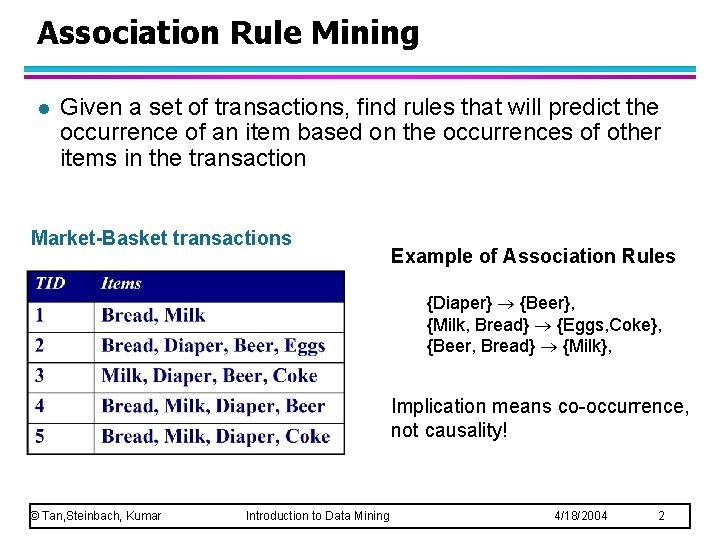
Association Rule Mining l Given a set of transactions, find rules that will predict the occurrence of an item based on the occurrences of other items in the transaction Market-Basket transactions Example of Association Rules {Diaper} {Beer}, {Milk, Bread} {Eggs, Coke}, {Beer, Bread} {Milk}, Implication means co-occurrence, not causality! © Tan, Steinbach, Kumar Introduction to Data Mining 4/18/2004 2

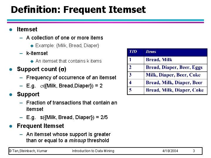
Definition: Frequent Itemset l Itemset – A collection of one or more items u Example: {Milk, Bread, Diaper} – k-itemset u l An itemset that contains k items Support count ( ) – Frequency of occurrence of an itemset – E. g. ({Milk, Bread, Diaper}) = 2 l Support – Fraction of transactions that contain an itemset – E. g. s({Milk, Bread, Diaper}) = 2/5 l Frequent Itemset – An itemset whose support is greater than or equal to a minsup threshold © Tan, Steinbach, Kumar Introduction to Data Mining 4/18/2004 3

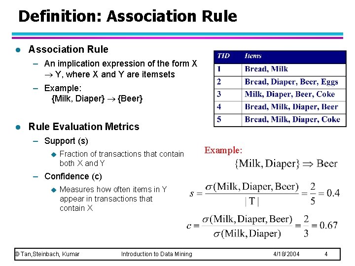
Definition: Association Rule l Association Rule – An implication expression of the form X Y, where X and Y are itemsets – Example: {Milk, Diaper} {Beer} l Rule Evaluation Metrics – Support (s) u Fraction of transactions that contain both X and Y Example: – Confidence (c) u Measures how often items in Y appear in transactions that contain X © Tan, Steinbach, Kumar Introduction to Data Mining 4/18/2004 4

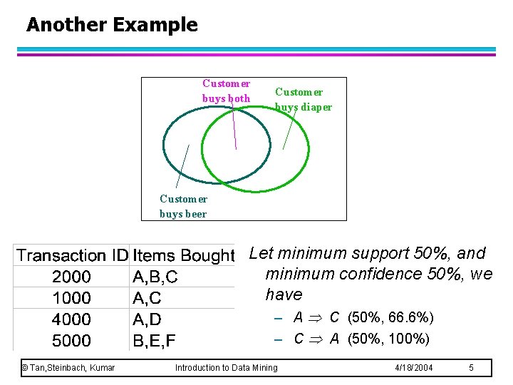
Another Example Customer buys both Customer buys diaper Customer buys beer Let minimum support 50%, and minimum confidence 50%, we have – A C (50%, 66. 6%) – C A (50%, 100%) © Tan, Steinbach, Kumar Introduction to Data Mining 4/18/2004 5

Association Rule Mining Task l Given a set of transactions T, the goal of association rule mining is to find all rules having – support ≥ minsup threshold – confidence ≥ minconf threshold l Brute-force approach: – List all possible association rules – Compute the support and confidence for each rule – Prune rules that fail the minsup and minconf thresholds Computationally prohibitive! © Tan, Steinbach, Kumar Introduction to Data Mining 4/18/2004 6

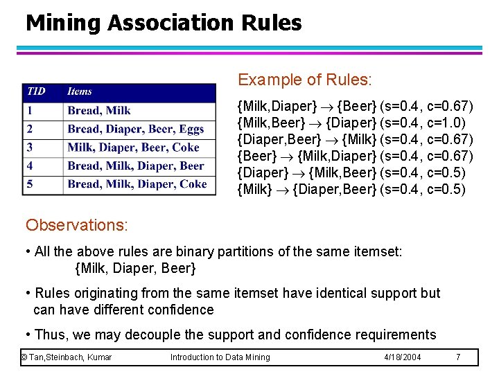
Mining Association Rules Example of Rules: {Milk, Diaper} {Beer} (s=0. 4, c=0. 67) {Milk, Beer} {Diaper} (s=0. 4, c=1. 0) {Diaper, Beer} {Milk} (s=0. 4, c=0. 67) {Beer} {Milk, Diaper} (s=0. 4, c=0. 67) {Diaper} {Milk, Beer} (s=0. 4, c=0. 5) {Milk} {Diaper, Beer} (s=0. 4, c=0. 5) Observations: • All the above rules are binary partitions of the same itemset: {Milk, Diaper, Beer} • Rules originating from the same itemset have identical support but can have different confidence • Thus, we may decouple the support and confidence requirements © Tan, Steinbach, Kumar Introduction to Data Mining 4/18/2004 7

Mining Association Rules l Two-step approach: 1. Frequent Itemset Generation – Generate all itemsets whose support minsup 2. Rule Generation – l Generate high confidence rules from each frequent itemset, where each rule is a binary partitioning of a frequent itemset Frequent itemset generation is still computationally expensive © Tan, Steinbach, Kumar Introduction to Data Mining 4/18/2004 8

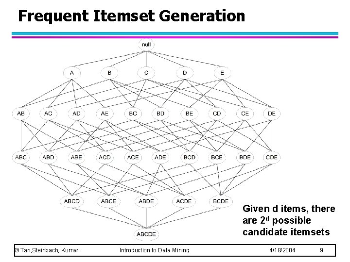
Frequent Itemset Generation Given d items, there are 2 d possible candidate itemsets © Tan, Steinbach, Kumar Introduction to Data Mining 4/18/2004 9

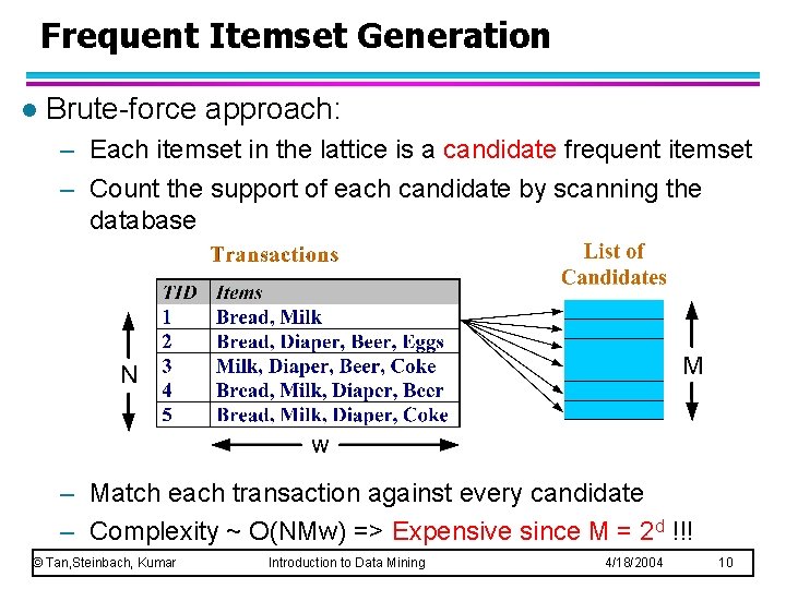
Frequent Itemset Generation l Brute-force approach: – Each itemset in the lattice is a candidate frequent itemset – Count the support of each candidate by scanning the database – Match each transaction against every candidate – Complexity ~ O(NMw) => Expensive since M = 2 d !!! © Tan, Steinbach, Kumar Introduction to Data Mining 4/18/2004 10

Frequent Itemset Generation Strategies l Reduce the number of candidates (M) – Complete search: M=2 d – Use pruning techniques to reduce M l Reduce the number of transactions (N) – Reduce size of N as the size of itemset increases l Reduce the number of comparisons (NM) – Use efficient data structures to store the candidates or transactions – No need to match every candidate against every transaction © Tan, Steinbach, Kumar Introduction to Data Mining 4/18/2004 11

Reducing Number of Candidates l Apriori principle: – If an itemset is frequent, then all of its subsets must also be frequent l Apriori principle holds due to the following property of the support measure: – Support of an itemset never exceeds the support of its subsets – This is known as the anti-monotone property of support © Tan, Steinbach, Kumar Introduction to Data Mining 4/18/2004 12

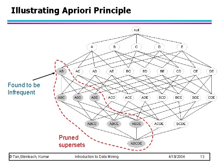
Illustrating Apriori Principle Found to be Infrequent Pruned supersets © Tan, Steinbach, Kumar Introduction to Data Mining 4/18/2004 13

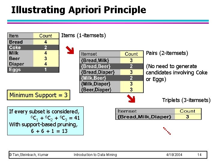
Illustrating Apriori Principle Items (1 -itemsets) Pairs (2 -itemsets) (No need to generate candidates involving Coke or Eggs) Minimum Support = 3 Triplets (3 -itemsets) If every subset is considered, 6 C + 6 C = 41 1 2 3 With support-based pruning, 6 + 1 = 13 © Tan, Steinbach, Kumar Introduction to Data Mining 4/18/2004 14

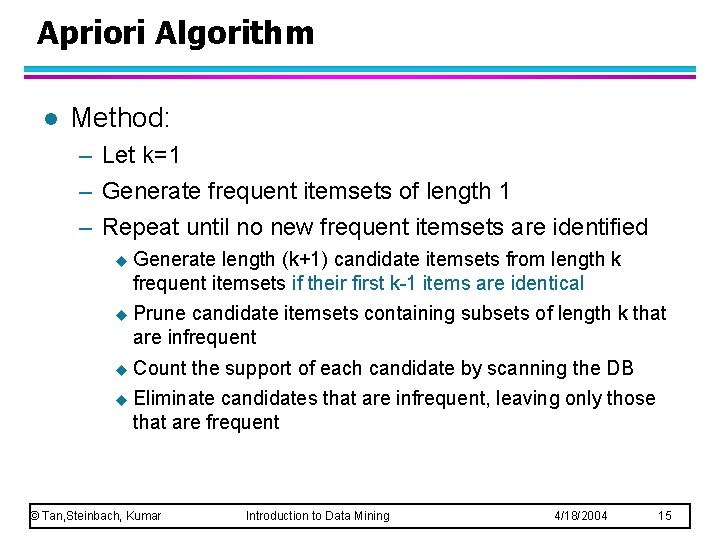
Apriori Algorithm l Method: – Let k=1 – Generate frequent itemsets of length 1 – Repeat until no new frequent itemsets are identified u Generate length (k+1) candidate itemsets from length k frequent itemsets if their first k-1 items are identical u Prune candidate itemsets containing subsets of length k that are infrequent u Count the support of each candidate by scanning the DB u Eliminate candidates that are infrequent, leaving only those that are frequent © Tan, Steinbach, Kumar Introduction to Data Mining 4/18/2004 15

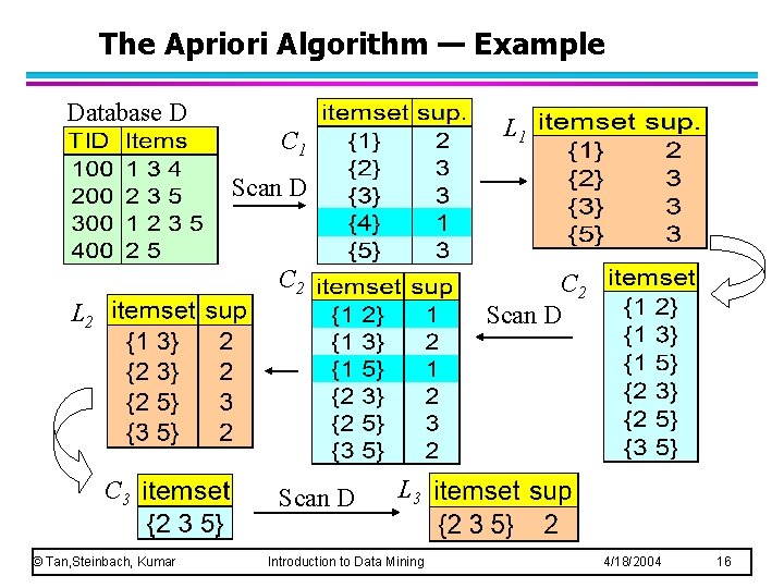
The Apriori Algorithm — Example Database D L 1 C 1 Scan D C 2 Scan D L 2 C 3 © Tan, Steinbach, Kumar Scan D L 3 Introduction to Data Mining 4/18/2004 16

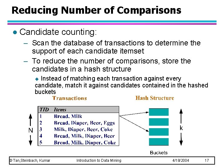
Reducing Number of Comparisons l Candidate counting: – Scan the database of transactions to determine the support of each candidate itemset – To reduce the number of comparisons, store the candidates in a hash structure Instead of matching each transaction against every candidate, match it against candidates contained in the hashed buckets u © Tan, Steinbach, Kumar Introduction to Data Mining 4/18/2004 17

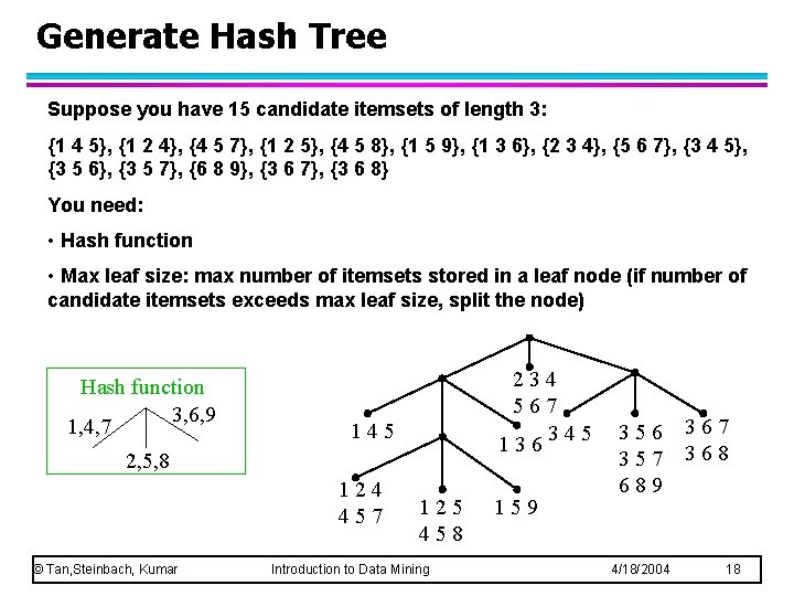
Generate Hash Tree Suppose you have 15 candidate itemsets of length 3: {1 4 5}, {1 2 4}, {4 5 7}, {1 2 5}, {4 5 8}, {1 5 9}, {1 3 6}, {2 3 4}, {5 6 7}, {3 4 5}, {3 5 6}, {3 5 7}, {6 8 9}, {3 6 7}, {3 6 8} You need: • Hash function • Max leaf size: max number of itemsets stored in a leaf node (if number of candidate itemsets exceeds max leaf size, split the node) Hash function 3, 6, 9 1, 4, 7 234 567 345 136 145 2, 5, 8 124 457 © Tan, Steinbach, Kumar 125 458 Introduction to Data Mining 159 356 357 689 4/18/2004 367 368 18

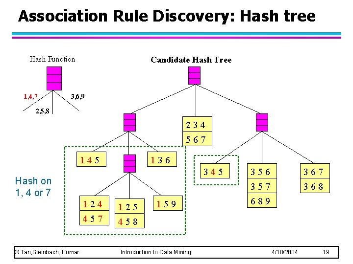
Association Rule Discovery: Hash tree Hash Function 1, 4, 7 Candidate Hash Tree 3, 6, 9 2, 5, 8 234 567 145 136 345 Hash on 1, 4 or 7 © Tan, Steinbach, Kumar 124 125 457 458 159 Introduction to Data Mining 356 367 368 357 689 4/18/2004 19

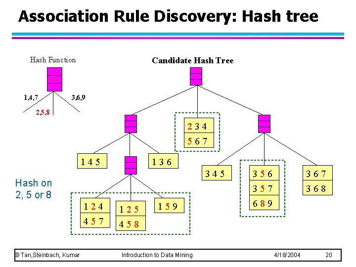
Association Rule Discovery: Hash tree Hash Function 1, 4, 7 Candidate Hash Tree 3, 6, 9 2, 5, 8 234 567 145 136 345 Hash on 2, 5 or 8 © Tan, Steinbach, Kumar 124 125 457 458 159 Introduction to Data Mining 356 367 368 357 689 4/18/2004 20

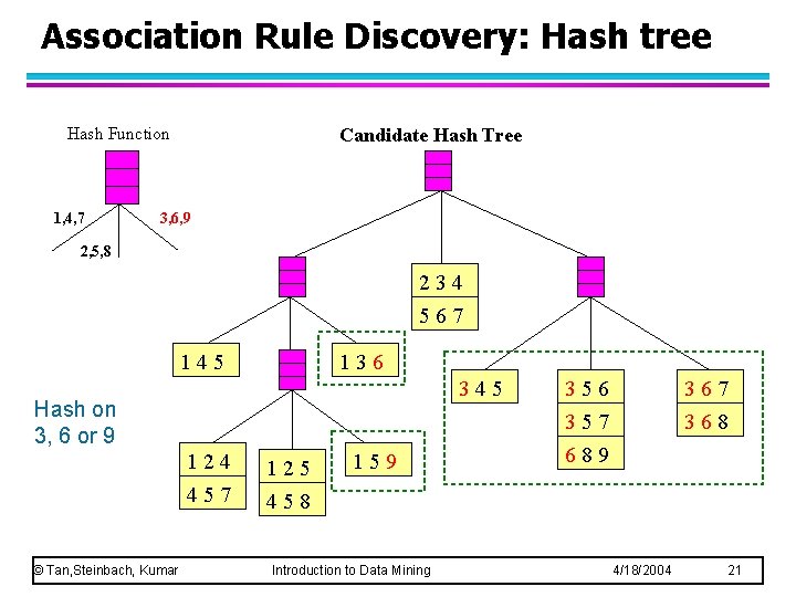
Association Rule Discovery: Hash tree Hash Function 1, 4, 7 Candidate Hash Tree 3, 6, 9 2, 5, 8 234 567 145 136 345 Hash on 3, 6 or 9 © Tan, Steinbach, Kumar 124 125 457 458 159 Introduction to Data Mining 356 367 368 357 689 4/18/2004 21

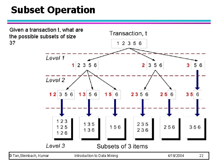
Subset Operation Given a transaction t, what are the possible subsets of size 3? © Tan, Steinbach, Kumar Introduction to Data Mining 4/18/2004 22

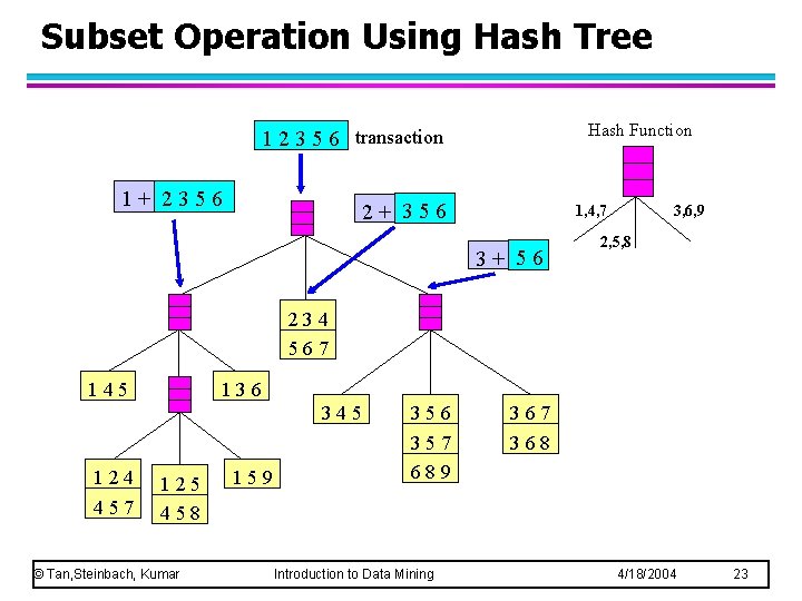
Subset Operation Using Hash Tree Hash Function 1 2 3 5 6 transaction 1+ 2356 2+ 356 1, 4, 7 3+ 56 3, 6, 9 2, 5, 8 234 567 145 136 345 124 457 125 458 © Tan, Steinbach, Kumar 159 356 357 689 Introduction to Data Mining 367 368 4/18/2004 23

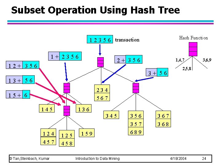
Subset Operation Using Hash Tree Hash Function 1 2 3 5 6 transaction 1+ 2356 2+ 356 1, 4, 7 3+ 56 3, 6, 9 2, 5, 8 13+ 56 234 567 15+ 6 145 136 345 124 457 © Tan, Steinbach, Kumar 125 458 159 Introduction to Data Mining 356 357 689 367 368 4/18/2004 24

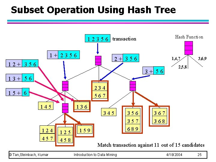
Subset Operation Using Hash Tree Hash Function 1 2 3 5 6 transaction 1+ 2356 2+ 356 1, 4, 7 3+ 56 3, 6, 9 2, 5, 8 13+ 56 234 567 15+ 6 145 136 345 124 457 © Tan, Steinbach, Kumar 125 458 159 356 357 689 367 368 Match transaction against 11 out of 15 candidates Introduction to Data Mining 4/18/2004 25

Factors Affecting Complexity l Choice of minimum support threshold – – l Dimensionality (number of items) of the data set – – l more space is needed to store support count of each item if number of frequent items also increases, both computation and I/O costs may also increase Size of database – l lowering support threshold results in more frequent itemsets this may increase number of candidates and max length of frequent itemsets since Apriori makes multiple passes, run time of algorithm may increase with number of transactions Average transaction width – transaction width increases with denser data sets – This may increase max length of frequent itemsets and traversals of hash tree (number of subsets in a transaction increases with its width) © Tan, Steinbach, Kumar Introduction to Data Mining 4/18/2004 26

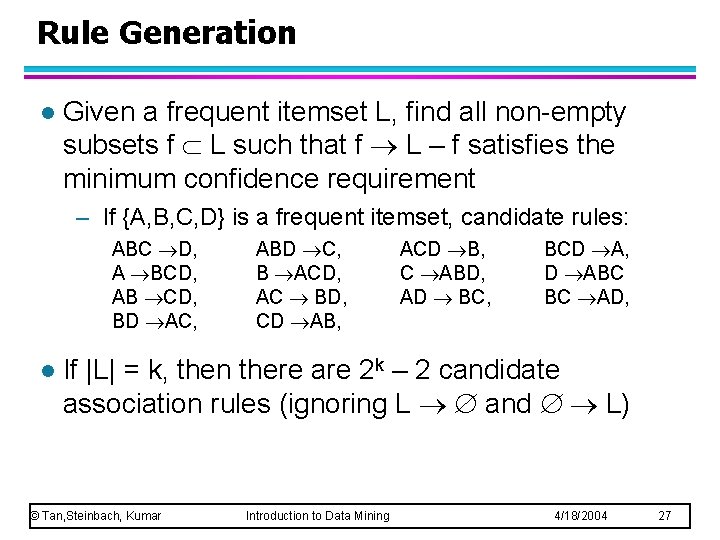
Rule Generation l Given a frequent itemset L, find all non-empty subsets f L such that f L – f satisfies the minimum confidence requirement – If {A, B, C, D} is a frequent itemset, candidate rules: ABC D, A BCD, AB CD, BD AC, l ABD C, B ACD, AC BD, CD AB, ACD B, C ABD, AD BC, BCD A, D ABC BC AD, If |L| = k, then there are 2 k – 2 candidate association rules (ignoring L and L) © Tan, Steinbach, Kumar Introduction to Data Mining 4/18/2004 27

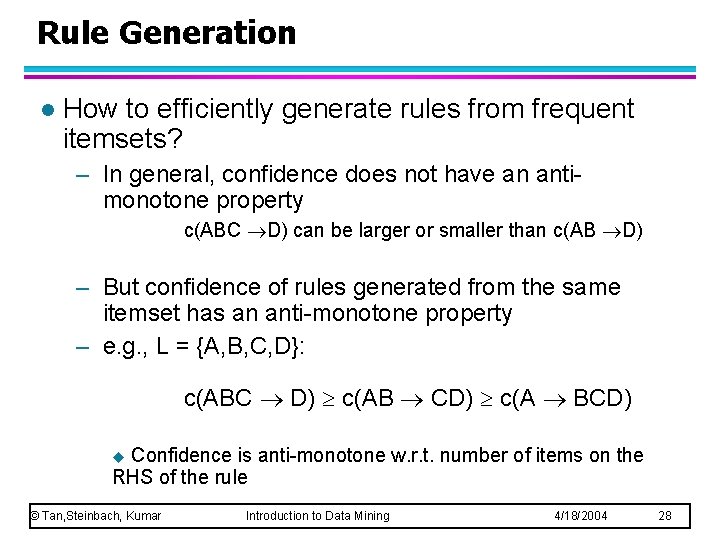
Rule Generation l How to efficiently generate rules from frequent itemsets? – In general, confidence does not have an antimonotone property c(ABC D) can be larger or smaller than c(AB D) – But confidence of rules generated from the same itemset has an anti-monotone property – e. g. , L = {A, B, C, D}: c(ABC D) c(AB CD) c(A BCD) Confidence is anti-monotone w. r. t. number of items on the RHS of the rule u © Tan, Steinbach, Kumar Introduction to Data Mining 4/18/2004 28

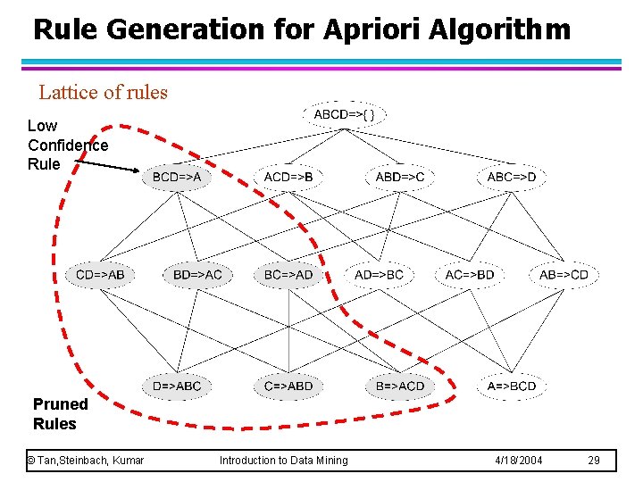
Rule Generation for Apriori Algorithm Lattice of rules Low Confidence Rule Pruned Rules © Tan, Steinbach, Kumar Introduction to Data Mining 4/18/2004 29

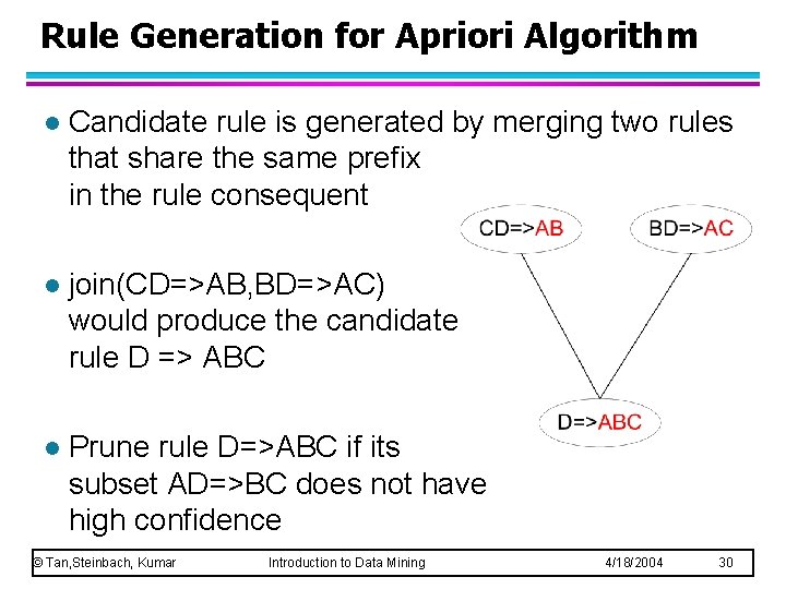
Rule Generation for Apriori Algorithm l Candidate rule is generated by merging two rules that share the same prefix in the rule consequent l join(CD=>AB, BD=>AC) would produce the candidate rule D => ABC l Prune rule D=>ABC if its subset AD=>BC does not have high confidence © Tan, Steinbach, Kumar Introduction to Data Mining 4/18/2004 30

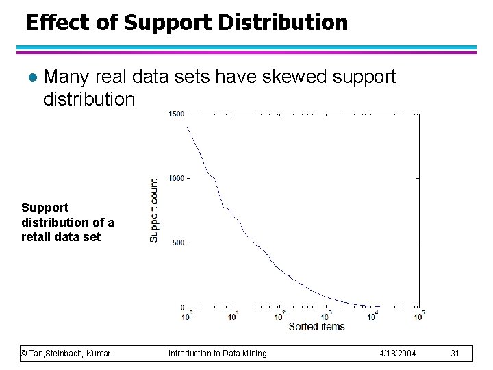
Effect of Support Distribution l Many real data sets have skewed support distribution Support distribution of a retail data set © Tan, Steinbach, Kumar Introduction to Data Mining 4/18/2004 31

Effect of Support Distribution l How to set the appropriate minsup threshold? – If minsup is set too high, we could miss itemsets involving interesting rare items (e. g. , expensive products) – If minsup is set too low, it is computationally expensive and the number of itemsets is very large l Using a single minimum support threshold may not be effective l Solution: use multiple minimum support, so a larger minsup for frequent items (e. g. , milk, bread) and a smaller minsup for rare items (e. g. , diamond) © Tan, Steinbach, Kumar Introduction to Data Mining 4/18/2004 32

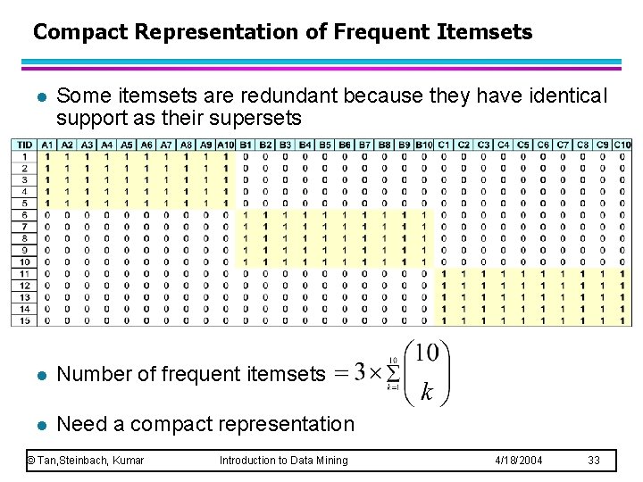
Compact Representation of Frequent Itemsets l Some itemsets are redundant because they have identical support as their supersets l Number of frequent itemsets l Need a compact representation © Tan, Steinbach, Kumar Introduction to Data Mining 4/18/2004 33

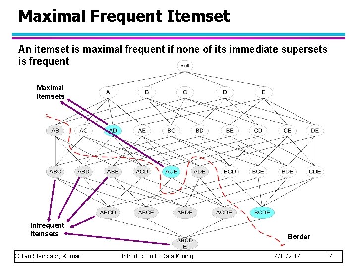
Maximal Frequent Itemset An itemset is maximal frequent if none of its immediate supersets is frequent Maximal Itemsets Infrequent Itemsets © Tan, Steinbach, Kumar Border Introduction to Data Mining 4/18/2004 34

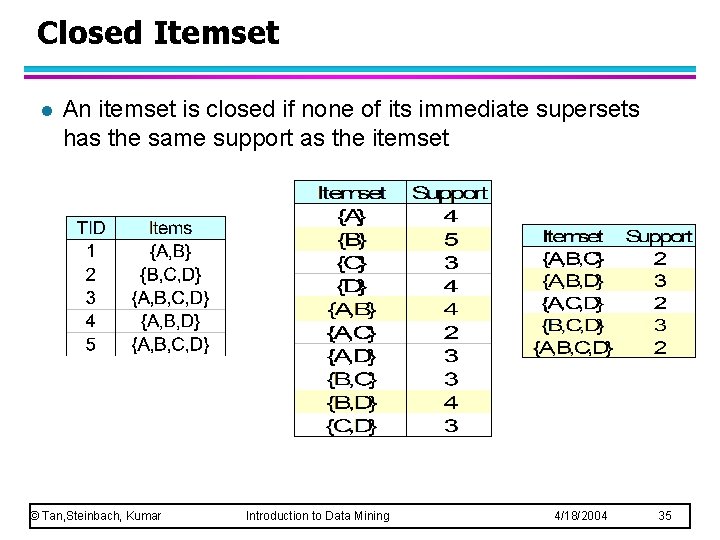
Closed Itemset l An itemset is closed if none of its immediate supersets has the same support as the itemset © Tan, Steinbach, Kumar Introduction to Data Mining 4/18/2004 35

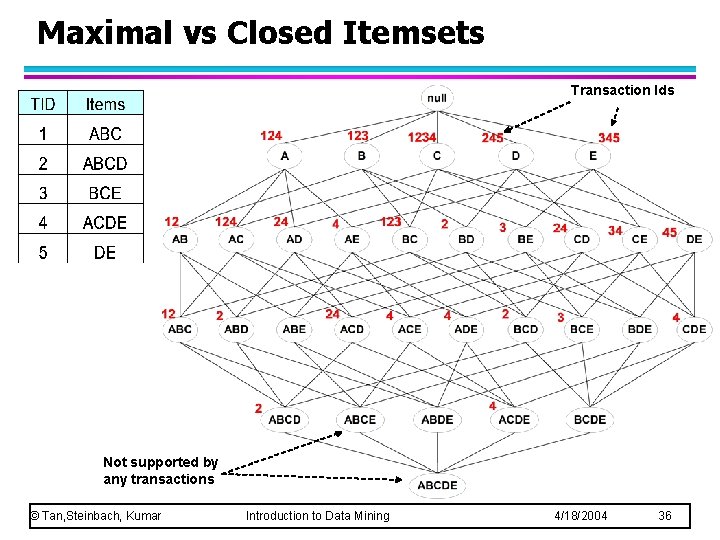
Maximal vs Closed Itemsets Transaction Ids Not supported by any transactions © Tan, Steinbach, Kumar Introduction to Data Mining 4/18/2004 36

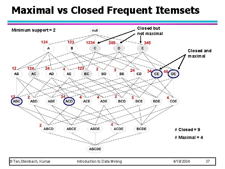
Maximal vs Closed Frequent Itemsets Closed but not maximal Minimum support = 2 Closed and maximal # Closed = 9 # Maximal = 4 © Tan, Steinbach, Kumar Introduction to Data Mining 4/18/2004 37

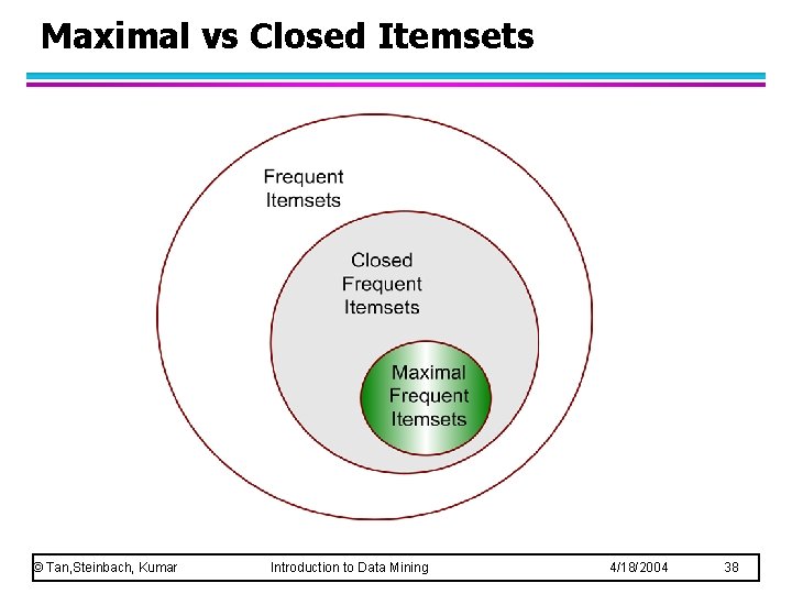
Maximal vs Closed Itemsets © Tan, Steinbach, Kumar Introduction to Data Mining 4/18/2004 38

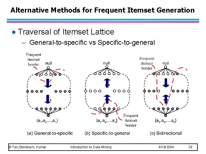
Alternative Methods for Frequent Itemset Generation l Traversal of Itemset Lattice – General-to-specific vs Specific-to-general © Tan, Steinbach, Kumar Introduction to Data Mining 4/18/2004 39

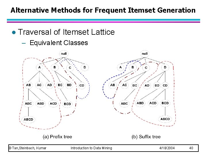
Alternative Methods for Frequent Itemset Generation l Traversal of Itemset Lattice – Equivalent Classes © Tan, Steinbach, Kumar Introduction to Data Mining 4/18/2004 40

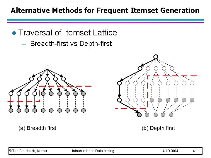
Alternative Methods for Frequent Itemset Generation l Traversal of Itemset Lattice – Breadth-first vs Depth-first © Tan, Steinbach, Kumar Introduction to Data Mining 4/18/2004 41

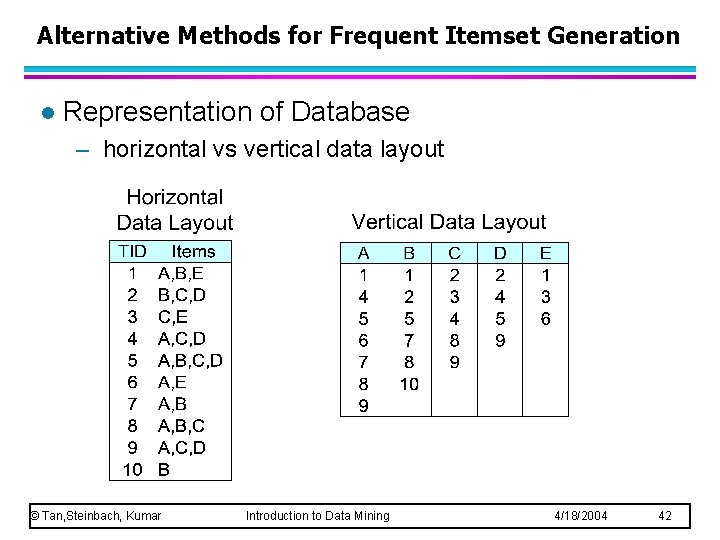
Alternative Methods for Frequent Itemset Generation l Representation of Database – horizontal vs vertical data layout © Tan, Steinbach, Kumar Introduction to Data Mining 4/18/2004 42

FP-growth Algorithm l Use a compressed representation of the database using an FP-tree l Once an FP-tree has been constructed, it uses a recursive divide-and-conquer approach to mine the frequent itemsets © Tan, Steinbach, Kumar Introduction to Data Mining 4/18/2004 43

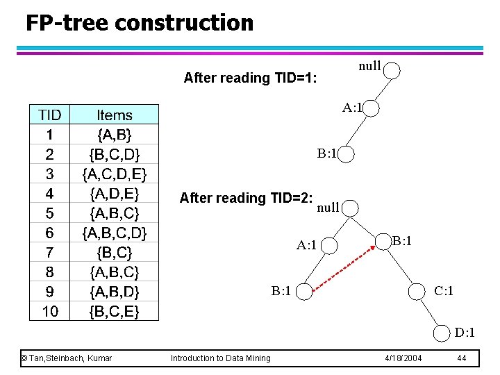
FP-tree construction null After reading TID=1: A: 1 B: 1 After reading TID=2: A: 1 null B: 1 C: 1 D: 1 © Tan, Steinbach, Kumar Introduction to Data Mining 4/18/2004 44

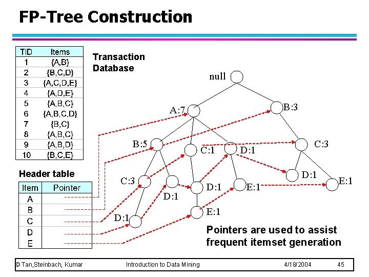
FP-Tree Construction Transaction Database null B: 3 A: 7 B: 5 Header table C: 1 C: 3 D: 1 D: 1 E: 1 Pointers are used to assist frequent itemset generation © Tan, Steinbach, Kumar Introduction to Data Mining 4/18/2004 45

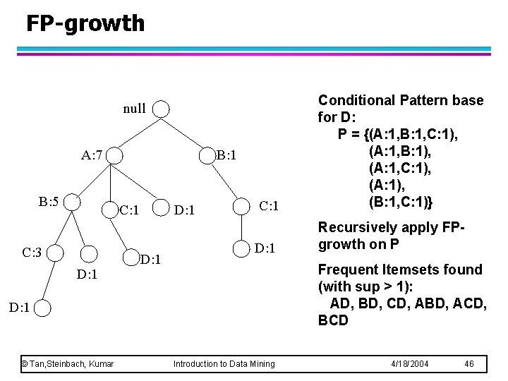
FP-growth C: 1 Conditional Pattern base for D: P = {(A: 1, B: 1, C: 1), (A: 1, B: 1), (A: 1, C: 1), (A: 1), (B: 1, C: 1)} D: 1 Recursively apply FPgrowth on P null A: 7 B: 5 B: 1 C: 3 D: 1 Frequent Itemsets found (with sup > 1): AD, BD, CD, ABD, ACD, BCD D: 1 © Tan, Steinbach, Kumar Introduction to Data Mining 4/18/2004 46

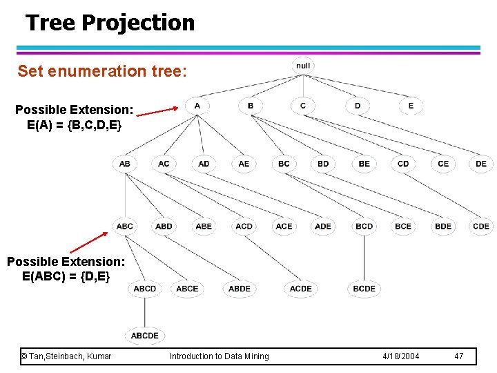
Tree Projection Set enumeration tree: Possible Extension: E(A) = {B, C, D, E} Possible Extension: E(ABC) = {D, E} © Tan, Steinbach, Kumar Introduction to Data Mining 4/18/2004 47

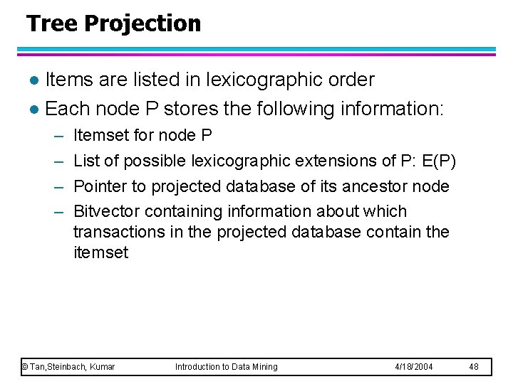
Tree Projection Items are listed in lexicographic order l Each node P stores the following information: l – – Itemset for node P List of possible lexicographic extensions of P: E(P) Pointer to projected database of its ancestor node Bitvector containing information about which transactions in the projected database contain the itemset © Tan, Steinbach, Kumar Introduction to Data Mining 4/18/2004 48

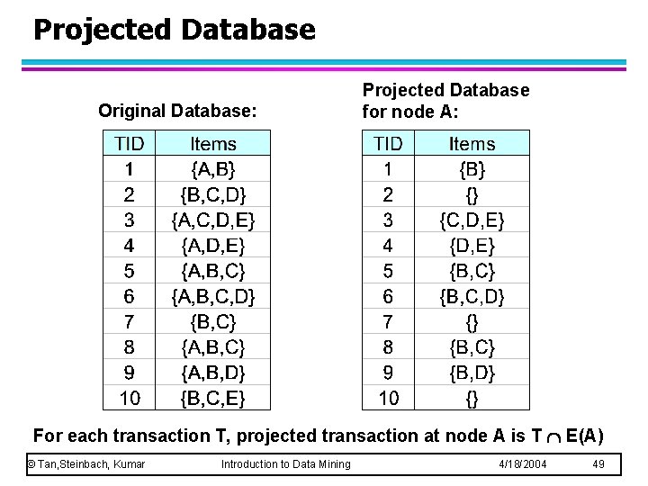
Projected Database Original Database: Projected Database for node A: For each transaction T, projected transaction at node A is T E(A) © Tan, Steinbach, Kumar Introduction to Data Mining 4/18/2004 49

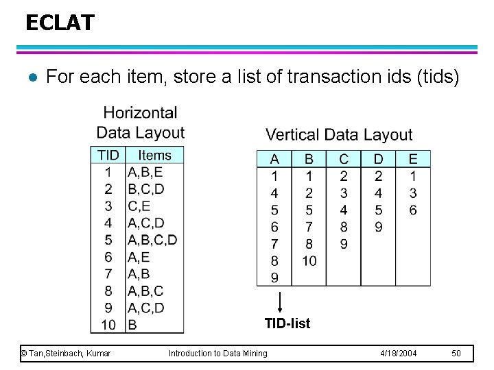
ECLAT l For each item, store a list of transaction ids (tids) TID-list © Tan, Steinbach, Kumar Introduction to Data Mining 4/18/2004 50

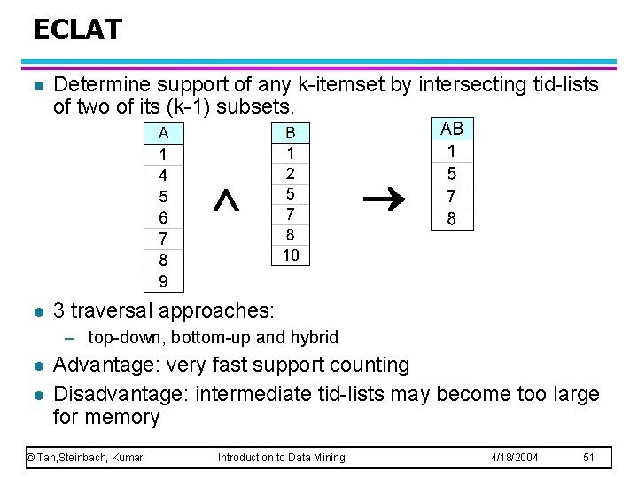
ECLAT l Determine support of any k-itemset by intersecting tid-lists of two of its (k-1) subsets. l 3 traversal approaches: – top-down, bottom-up and hybrid l l Advantage: very fast support counting Disadvantage: intermediate tid-lists may become too large for memory © Tan, Steinbach, Kumar Introduction to Data Mining 4/18/2004 51

Pattern Evaluation l Association rule algorithms tend to produce too many rules – many of them are uninteresting or redundant – Redundant if {A, B, C} {D} and {A, B} {D} have same support & confidence Interestingness measures can be used to prune/rank the derived patterns l In the original formulation of association rules, support & confidence are the only measures used an objective interestingness measure. l – An object interestingness measure is domain independent. © Tan, Steinbach, Kumar Introduction to Data Mining 4/18/2004 52

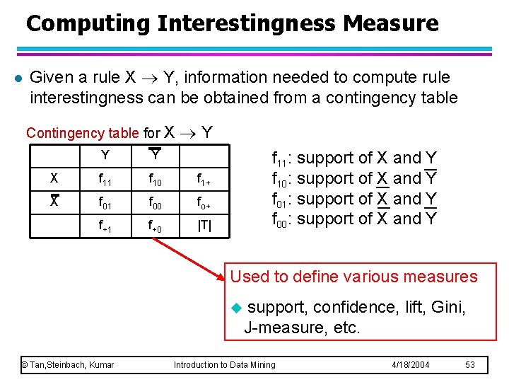
Computing Interestingness Measure l Given a rule X Y, information needed to compute rule interestingness can be obtained from a contingency table Contingency table for X Y Y Y X f 11 f 10 f 1+ X f 01 f 00 fo+ f+1 f+0 |T| f 11: support of X and Y f 10: support of X and Y f 01: support of X and Y f 00: support of X and Y Used to define various measures u © Tan, Steinbach, Kumar support, confidence, lift, Gini, J-measure, etc. Introduction to Data Mining 4/18/2004 53

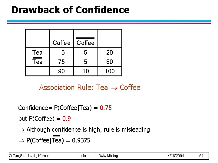
Drawback of Confidence Coffee Tea 15 5 20 Tea 75 5 80 90 10 100 Association Rule: Tea Coffee Confidence= P(Coffee|Tea) = 0. 75 but P(Coffee) = 0. 9 Although confidence is high, rule is misleading P(Coffee|Tea) = 0. 9375 © Tan, Steinbach, Kumar Introduction to Data Mining 4/18/2004 54

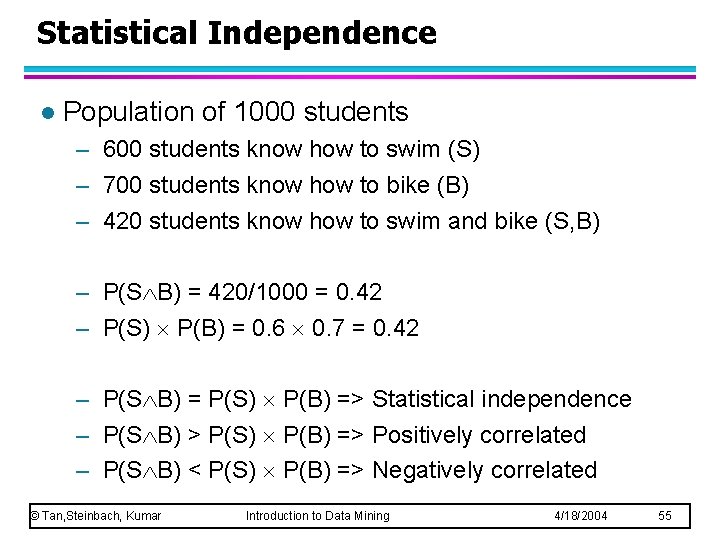
Statistical Independence l Population of 1000 students – 600 students know how to swim (S) – 700 students know how to bike (B) – 420 students know how to swim and bike (S, B) – P(S B) = 420/1000 = 0. 42 – P(S) P(B) = 0. 6 0. 7 = 0. 42 – P(S B) = P(S) P(B) => Statistical independence – P(S B) > P(S) P(B) => Positively correlated – P(S B) < P(S) P(B) => Negatively correlated © Tan, Steinbach, Kumar Introduction to Data Mining 4/18/2004 55

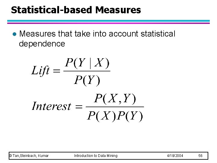
Statistical-based Measures l Measures that take into account statistical dependence © Tan, Steinbach, Kumar Introduction to Data Mining 4/18/2004 56

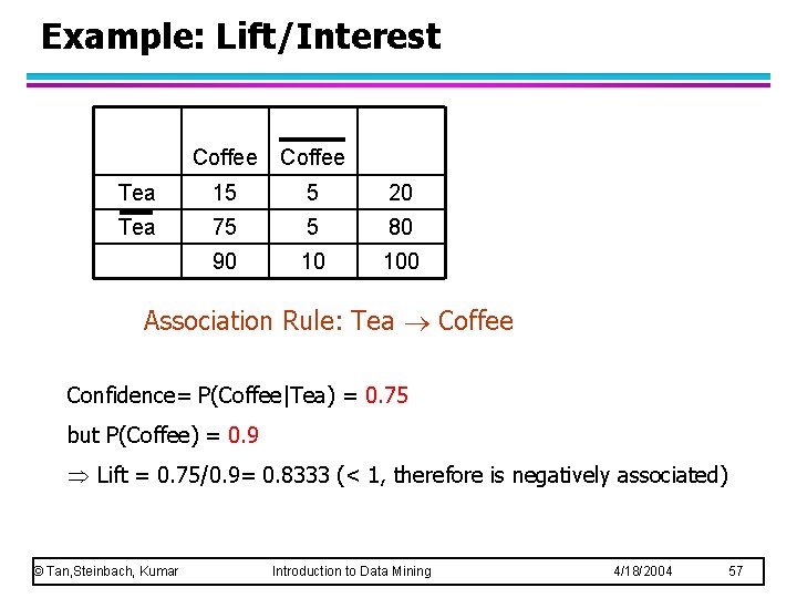
Example: Lift/Interest Coffee Tea 15 5 20 Tea 75 5 80 90 10 100 Association Rule: Tea Coffee Confidence= P(Coffee|Tea) = 0. 75 but P(Coffee) = 0. 9 Lift = 0. 75/0. 9= 0. 8333 (< 1, therefore is negatively associated) © Tan, Steinbach, Kumar Introduction to Data Mining 4/18/2004 57

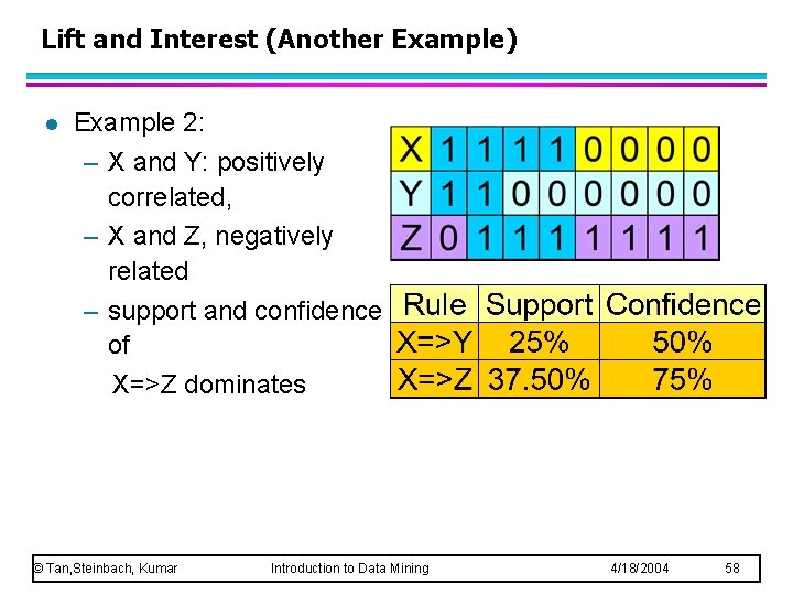
Lift and Interest (Another Example) l Example 2: – X and Y: positively correlated, – X and Z, negatively related – support and confidence of X=>Z dominates © Tan, Steinbach, Kumar Introduction to Data Mining 4/18/2004 58

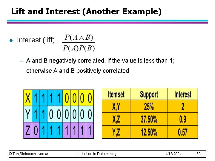
Lift and Interest (Another Example) l Interest (lift) – A and B negatively correlated, if the value is less than 1; otherwise A and B positively correlated © Tan, Steinbach, Kumar Introduction to Data Mining 4/18/2004 59

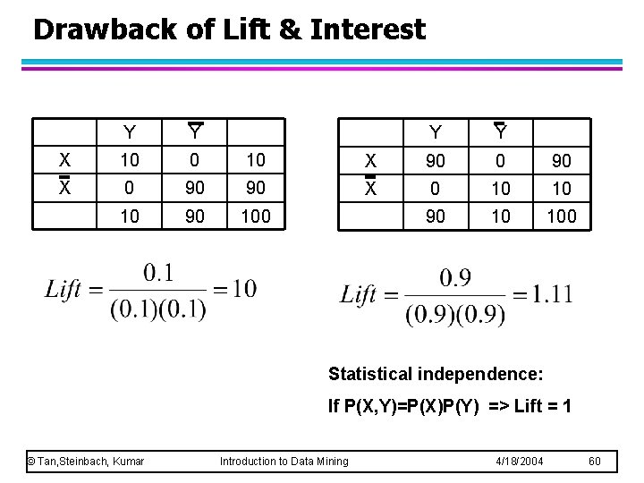
Drawback of Lift & Interest Y Y X 10 0 10 X 0 90 90 100 Y Y X 90 0 90 X 0 10 10 90 10 100 Statistical independence: If P(X, Y)=P(X)P(Y) => Lift = 1 © Tan, Steinbach, Kumar Introduction to Data Mining 4/18/2004 60

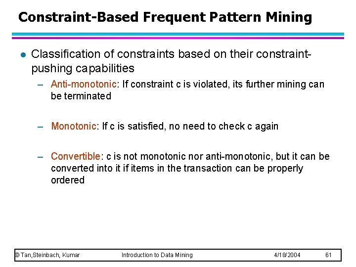
Constraint-Based Frequent Pattern Mining l Classification of constraints based on their constraintpushing capabilities – Anti-monotonic: If constraint c is violated, its further mining can be terminated – Monotonic: If c is satisfied, no need to check c again – Convertible: c is not monotonic nor anti-monotonic, but it can be converted into it if items in the transaction can be properly ordered © Tan, Steinbach, Kumar Introduction to Data Mining 4/18/2004 61

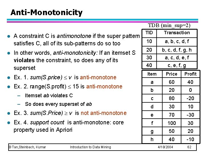
Anti-Monotonicity TDB (min_sup=2) l A constraint C is antimonotone if the super pattern satisfies C, all of its sub-patterns do so too l In other words, anti-monotonicity: If an itemset S violates the constraint, so does any of its superset l Ex. 1. sum(S. price) v is anti-monotone l Ex. 2. range(S. profit) 15 is anti-monotone – Itemset ab violates C – So does every superset of ab l Ex. 3. sum(S. Price) v is not anti-monotone l Ex. 4. support count is anti-monotone: core property used in Apriori © Tan, Steinbach, Kumar Introduction to Data Mining TID Transaction 10 a, b, c, d, f 20 30 40 b, c, d, f, g, h a, c, d, e, f c, e, f, g Item Price Profit a 60 40 b 20 0 c 80 -20 d 30 10 e 70 -30 f 100 30 g 50 20 h 40 -10 4/18/2004 62

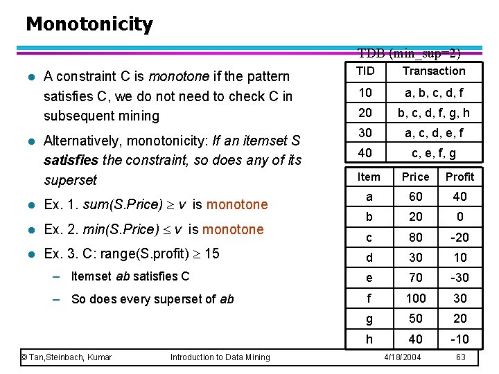
Monotonicity TDB (min_sup=2) l l A constraint C is monotone if the pattern satisfies C, we do not need to check C in subsequent mining Alternatively, monotonicity: If an itemset S satisfies the constraint, so does any of its superset TID Transaction 10 a, b, c, d, f 20 b, c, d, f, g, h 30 a, c, d, e, f 40 c, e, f, g Item Price Profit a 60 40 b 20 0 c 80 -20 d 30 10 – Itemset ab satisfies C e 70 -30 – So does every superset of ab f 100 30 g 50 20 h 40 -10 l Ex. 1. sum(S. Price) v is monotone l Ex. 2. min(S. Price) v is monotone l Ex. 3. C: range(S. profit) 15 © Tan, Steinbach, Kumar Introduction to Data Mining 4/18/2004 63

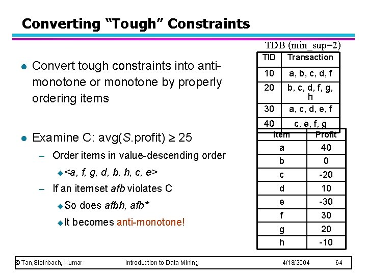
Converting “Tough” Constraints TDB (min_sup=2) l l Convert tough constraints into antimonotone or monotone by properly ordering items Examine C: avg(S. profit) 25 – Order items in value-descending order u<a, f, g, d, b, h, c, e> – If an itemset afb violates C u. So u. It does afbh, afb* becomes anti-monotone! © Tan, Steinbach, Kumar Introduction to Data Mining TID Transaction 10 a, b, c, d, f 20 30 b, c, d, f, g, h a, c, d, e, f 40 c, e, f, g Item Profit a b c d e f g h 40 0 -20 10 -30 30 20 -10 4/18/2004 64

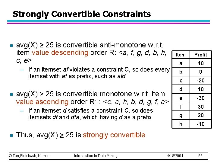
Strongly Convertible Constraints l avg(X) 25 is convertible anti-monotone w. r. t. item value descending order R: <a, f, g, d, b, h, c, e> – If an itemset af violates a constraint C, so does every itemset with af as prefix, such as afd l avg(X) 25 is convertible monotone w. r. t. item value ascending order R-1: <e, c, h, b, d, g, f, a> – If an itemset d satisfies a constraint C, so does itemsets df and dfa, which having d as a prefix l Item Profit a 40 b 0 c -20 d 10 e -30 f 30 g 20 h -10 Thus, avg(X) 25 is strongly convertible © Tan, Steinbach, Kumar Introduction to Data Mining 4/18/2004 65