Data Mining and Warehousing Unit V Bayesian Classification

Data Mining and Warehousing Unit - V

Bayesian Classification: Why? • A statistical classifier: performs probabilistic prediction, i. e. , predicts class membership probabilities • Foundation: Based on Bayes’ Theorem. • Performance: A simple Bayesian classifier, naïve Bayesian classifier, has comparable performance with decision tree and selected neural network classifiers • Incremental: Each training example can incrementally increase/decrease the probability that a hypothesis is correct — prior knowledge can be combined with observed data • Standard: Even when Bayesian methods are computationally intractable, they can provide a standard of optimal decision making against which other methods can be measured January 23, 2022 Data Mining: Concepts and Techniques 2

Bayesian Theorem: Basics • Let X be a data sample (“evidence”): class label is unknown • Let H be a hypothesis that X belongs to class C • Classification is to determine P(H|X), the probability that the hypothesis holds given the observed data sample X • P(H) (prior probability), the initial probability – E. g. , X will buy computer, regardless of age, income, … • P(X): probability that sample data is observed • P(X|H) (posteriori probability), the probability of observing the sample X, given that the hypothesis holds – E. g. , Given that X will buy computer, the prob. that X is 31. . 40, medium income January 23, 2022 Data Mining: Concepts and Techniques 3

Bayesian Theorem • Given training data X, posteriori probability of a hypothesis H, P(H|X), follows the Bayes theorem • Informally, this can be written as posteriori = likelihood x prior/evidence • Predicts X belongs to C 2 iff the probability P(Ci|X) is the highest among all the P(Ck|X) for all the k classes • Practical difficulty: require initial knowledge of many probabilities, significant computational cost January 23, 2022 Data Mining: Concepts and Techniques 4

Towards Naïve Bayesian Classifier • Let D be a training set of tuples and their associated class labels, and each tuple is represented by an n-D attribute vector X = (x 1, x 2, …, xn) • Suppose there are m classes C 1, C 2, …, Cm. • Classification is to derive the maximum posteriori, i. e. , the maximal P(Ci|X) • This can be derived from Bayes’ theorem • Since P(X) is constant for all classes, only needs to be maximized January 23, 2022 Data Mining: Concepts and Techniques 5

Derivation of Naïve Bayes Classifier • A simplified assumption: attributes are conditionally independent (i. e. , no dependence relation between attributes): • This greatly reduces the computation cost: Only counts the class distribution • If Ak is categorical, P(xk|Ci) is the # of tuples in Ci having value xk for Ak divided by |Ci, D| (# of tuples of Ci in D) • If Ak is continous-valued, P(xk|Ci) is usually computed based on Gaussian distribution with a mean μ and standard deviation σ and P(xk|Ci) is January 23, 2022 Data Mining: Concepts and Techniques 6

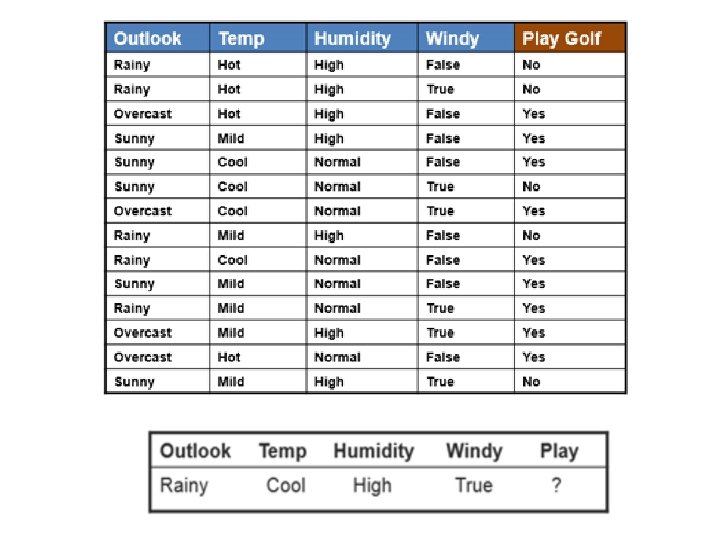
Naive Bayesian The Naive Bayesian classifier is based on Bayes’ theorem with the independence assumptions between predictors. A Naive Bayesian model is easy to build, with no complicated iterative parameter estimation which makes it particularly useful for very large datasets. Despite its simplicity, the Naive Bayesian classifier often does surprisingly well and is widely used because it often outperforms more sophisticated classification methods. Algorithm Bayes theorem provides a way of calculating the posterior probability, P(c|x), from P(c), P(x), and P(x|c). Naive Bayes classifier assume that the effect of the value of a predictor (x) on a given class (c) is independent of the values of other predictors. This assumption is called class conditional independence.

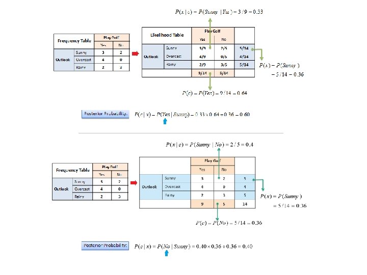
• P(c|x) is the posterior probability of class (target) given predictor (attribute). • P(c) is the prior probability of class. • P(x|c) is the likelihood which is the probability of predictor given class. • P(x) is the prior probability of predictor.

Naïve Bayesian Classifier: Training Dataset Class: C 1: buys_computer = ‘yes’ C 2: buys_computer = ‘no’ Data sample X = (age <=30, Income = medium, Student = yes Credit_rating = Fair) January 23, 2022 Data Mining: Concepts and Techniques 9

Naïve Bayesian Classifier: An Example • P(Ci): P(buys_computer = “yes”) = 9/14 = 0. 643 P(buys_computer = “no”) = 5/14= 0. 357 • Compute P(X|Ci) for each class P(age = “<=30” | buys_computer = “yes”) = 2/9 = 0. 222 P(age = “<= 30” | buys_computer = “no”) = 3/5 = 0. 6 P(income = “medium” | buys_computer = “yes”) = 4/9 = 0. 444 P(income = “medium” | buys_computer = “no”) = 2/5 = 0. 4 P(student = “yes” | buys_computer = “yes) = 6/9 = 0. 667 P(student = “yes” | buys_computer = “no”) = 1/5 = 0. 2 P(credit_rating = “fair” | buys_computer = “yes”) = 6/9 = 0. 667 P(credit_rating = “fair” | buys_computer = “no”) = 2/5 = 0. 4 • X = (age <= 30 , income = medium, student = yes, credit_rating = fair) P(X|Ci) : P(X|buys_computer = “yes”) = 0. 222 x 0. 444 x 0. 667 = 0. 044 P(X|buys_computer = “no”) = 0. 6 x 0. 4 x 0. 2 x 0. 4 = 0. 019 P(X|Ci)*P(Ci) : P(X|buys_computer = “yes”) * P(buys_computer = “yes”) = 0. 028 P(X|buys_computer = “no”) * P(buys_computer = “no”) = 0. 007 Therefore, X belongs to class (“buys_computer = yes”) January 23, 2022 Data Mining: Concepts and Techniques 10