Data Mining and machine learning DM Lecture 5

Data Mining (and machine learning) DM Lecture 5: Feature Selection

Today Recap/extra correlation/regression: Feature Selection: More on Coursework 2

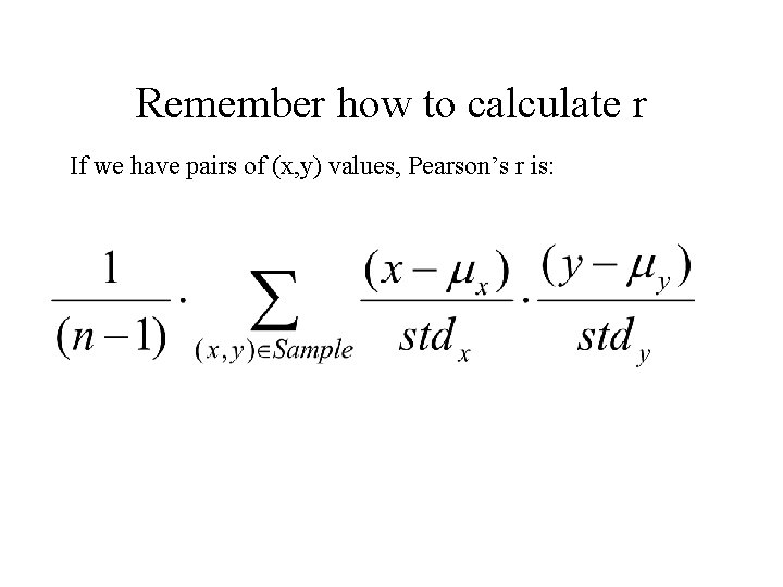
Remember how to calculate r If we have pairs of (x, y) values, Pearson’s r is:

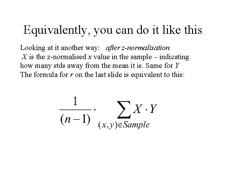
Equivalently, you can do it like this Looking at it another way: after z-normalisation X is the z-normalised x value in the sample – indicating how many stds away from the mean it is. Same for Y The formula for r on the last slide is equivalent to this:

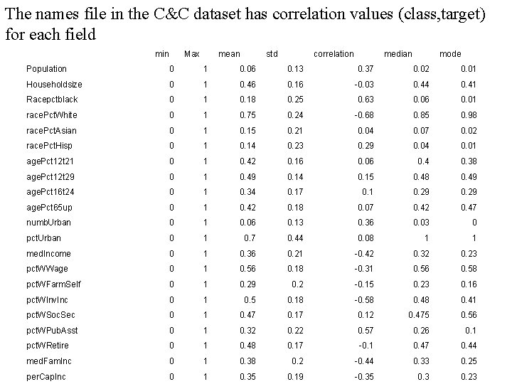
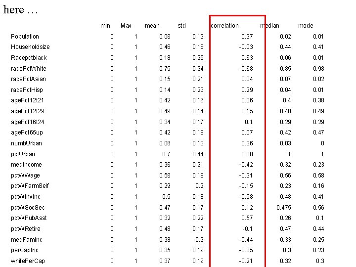
The names file in the C&C dataset has correlation values (class, target) for each field min Max mean std correlation median mode Population 0 1 0. 06 0. 13 0. 37 0. 02 0. 01 Householdsize 0 1 0. 46 0. 16 -0. 03 0. 44 0. 41 Racepctblack 0 1 0. 18 0. 25 0. 63 0. 06 0. 01 race. Pct. White 0 1 0. 75 0. 24 -0. 68 0. 85 0. 98 race. Pct. Asian 0 1 0. 15 0. 21 0. 04 0. 07 0. 02 race. Pct. Hisp 0 1 0. 14 0. 23 0. 29 0. 04 0. 01 age. Pct 12 t 21 0 1 0. 42 0. 16 0. 06 0. 4 0. 38 age. Pct 12 t 29 0 1 0. 49 0. 14 0. 15 0. 48 0. 49 age. Pct 16 t 24 0 1 0. 34 0. 17 0. 1 0. 29 age. Pct 65 up 0 1 0. 42 0. 18 0. 07 0. 42 0. 47 numb. Urban 0 1 0. 06 0. 13 0. 36 0. 03 0 pct. Urban 0 1 0. 7 0. 44 0. 08 1 1 med. Income 0 1 0. 36 0. 21 -0. 42 0. 32 0. 23 pct. WWage 0 1 0. 56 0. 18 -0. 31 0. 56 0. 58 pct. WFarm. Self 0 1 0. 29 0. 2 -0. 15 0. 23 0. 16 pct. WInv. Inc 0 1 0. 5 0. 18 -0. 58 0. 41 pct. WSoc. Sec 0 1 0. 47 0. 12 0. 475 0. 56 pct. WPub. Asst 0 1 0. 32 0. 22 0. 57 0. 26 0. 1 pct. WRetire 0 1 0. 48 0. 17 -0. 1 0. 47 0. 44 med. Fam. Inc 0 1 0. 38 0. 2 -0. 44 0. 33 0. 25 per. Cap. Inc 0 1 0. 35 0. 19 -0. 35 0. 3 0. 23

here … min Max mean std correlation median mode Population 0 1 0. 06 0. 13 0. 37 0. 02 0. 01 Householdsize 0 1 0. 46 0. 16 -0. 03 0. 44 0. 41 Racepctblack 0 1 0. 18 0. 25 0. 63 0. 06 0. 01 race. Pct. White 0 1 0. 75 0. 24 -0. 68 0. 85 0. 98 race. Pct. Asian 0 1 0. 15 0. 21 0. 04 0. 07 0. 02 race. Pct. Hisp 0 1 0. 14 0. 23 0. 29 0. 04 0. 01 age. Pct 12 t 21 0 1 0. 42 0. 16 0. 06 0. 4 0. 38 age. Pct 12 t 29 0 1 0. 49 0. 14 0. 15 0. 48 0. 49 age. Pct 16 t 24 0 1 0. 34 0. 17 0. 1 0. 29 age. Pct 65 up 0 1 0. 42 0. 18 0. 07 0. 42 0. 47 numb. Urban 0 1 0. 06 0. 13 0. 36 0. 03 0 pct. Urban 0 1 0. 7 0. 44 0. 08 1 1 med. Income 0 1 0. 36 0. 21 -0. 42 0. 32 0. 23 pct. WWage 0 1 0. 56 0. 18 -0. 31 0. 56 0. 58 pct. WFarm. Self 0 1 0. 29 0. 2 -0. 15 0. 23 0. 16 pct. WInv. Inc 0 1 0. 5 0. 18 -0. 58 0. 41 pct. WSoc. Sec 0 1 0. 47 0. 12 0. 475 0. 56 pct. WPub. Asst 0 1 0. 32 0. 22 0. 57 0. 26 0. 1 pct. WRetire 0 1 0. 48 0. 17 -0. 1 0. 47 0. 44 med. Fam. Inc 0 1 0. 38 0. 2 -0. 44 0. 33 0. 25 per. Cap. Inc 0 1 0. 35 0. 19 -0. 35 0. 3 0. 23 white. Per. Cap 0 1 0. 37 0. 19 -0. 21 0. 32 0. 3

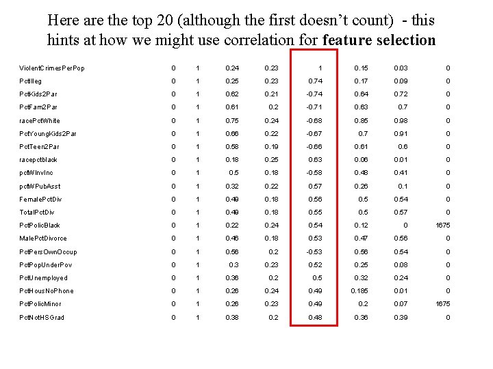
Here are the top 20 (although the first doesn’t count) - this hints at how we might use correlation for feature selection Violent. Crimes. Per. Pop 0 1 0. 24 0. 23 1 0. 15 0. 03 0 Pct. Illeg 0 1 0. 25 0. 23 0. 74 0. 17 0. 09 0 Pct. Kids 2 Par 0 1 0. 62 0. 21 -0. 74 0. 64 0. 72 0 Pct. Fam 2 Par 0 1 0. 61 0. 2 -0. 71 0. 63 0. 7 0 race. Pct. White 0 1 0. 75 0. 24 -0. 68 0. 85 0. 98 0 Pct. Young. Kids 2 Par 0 1 0. 66 0. 22 -0. 67 0. 91 0 Pct. Teen 2 Par 0 1 0. 58 0. 19 -0. 66 0. 61 0. 6 0 racepctblack 0 1 0. 18 0. 25 0. 63 0. 06 0. 01 0 pct. WInv. Inc 0 1 0. 5 0. 18 -0. 58 0. 41 0 pct. WPub. Asst 0 1 0. 32 0. 22 0. 57 0. 26 0. 1 0 Female. Pct. Div 0 1 0. 49 0. 18 0. 56 0. 54 0 Total. Pct. Div 0 1 0. 49 0. 18 0. 55 0. 57 0 Pct. Polic. Black 0 1 0. 22 0. 24 0. 54 0. 12 0 1675 Male. Pct. Divorce 0 1 0. 46 0. 18 0. 53 0. 47 0. 56 0 Pct. Pers. Own. Occup 0 1 0. 56 0. 2 -0. 53 0. 56 0. 54 0 Pct. Pop. Under. Pov 0 1 0. 3 0. 23 0. 52 0. 25 0. 08 0 Pct. Unemployed 0 1 0. 36 0. 2 0. 5 0. 32 0. 24 0 Pct. Hous. No. Phone 0 1 0. 26 0. 24 0. 49 0. 185 0. 01 0 Pct. Polic. Minor 0 1 0. 26 0. 23 0. 49 0. 2 0. 07 1675 Pct. Not. HSGrad 0 1 0. 38 0. 2 0. 48 0. 36 0. 39 0

Can anyone see a potential problem with choosing only (for example) the 20 features that correlate best with the target class ?

Feature Selection: What You have some data, and you want to use it to build a classifier, so that you can predict something (e. g. likelihood of cancer)

Feature Selection: What You have some data, and you want to use it to build a classifier, so that you can predict something (e. g. likelihood of cancer) The data has 10, 000 fields (features)

Feature Selection: What You have some data, and you want to use it to build a classifier, so that you can predict something (e. g. likelihood of cancer) The data has 10, 000 fields (features) you need to cut it down to 1, 000 fields before you try machine learning. Which 1, 000?

Feature Selection: What You have some data, and you want to use it to build a classifier, so that you can predict something (e. g. likelihood of cancer) The data has 10, 000 fields (features) you need to cut it down to 1, 000 fields before you try machine learning. Which 1, 000? The process of choosing the 1, 000 fields to use is called Feature Selection

Datasets with many features Gene expression datasets (~10, 000 features) http: //www. ncbi. nlm. nih. gov/sites/entrez? db=gds Proteomics data (~20, 000 features) http: //www. ebi. ac. uk/pride/ Satellite image data … Weather data …. .

Feature Selection: Why?

Feature Selection: Why?

Feature Selection: Why? From http: //elpub. scix. net/data/works/att/02 -28. content. pdf

Quite easy to find lots more cases from papers, where experiments show that accuracy reduces when you use more features

• Why does accuracy reduce with more features? • How does it depend on the specific choice of features? • What else changes if we use more features? • So, how do we choose the right features?

Why accuracy reduces: • Note: suppose the best feature set has 20 features. If you add another 5 features, typically the accuracy of machine learning may reduce. But you still have the original 20 features!! Why does this happen? ? ?

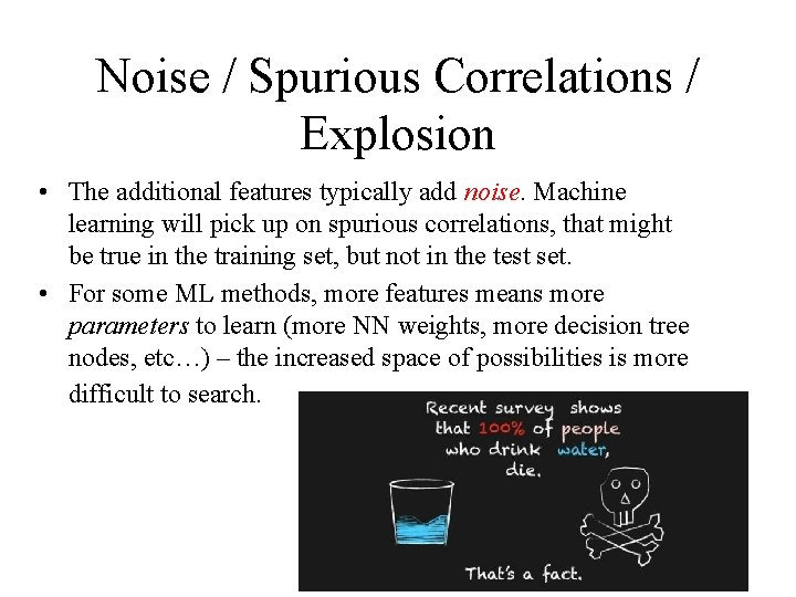
Noise / Spurious Correlations / Explosion • The additional features typically add noise. Machine learning will pick up on spurious correlations, that might be true in the training set, but not in the test set. • For some ML methods, more features means more parameters to learn (more NN weights, more decision tree nodes, etc…) – the increased space of possibilities is more difficult to search.

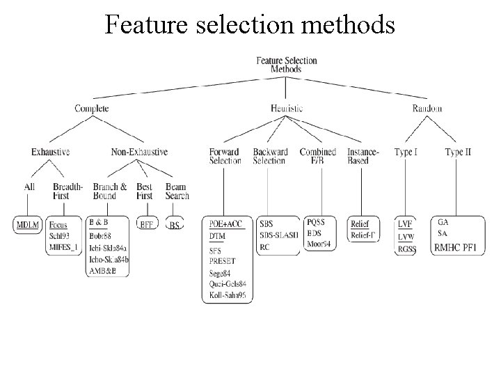
Feature selection methods

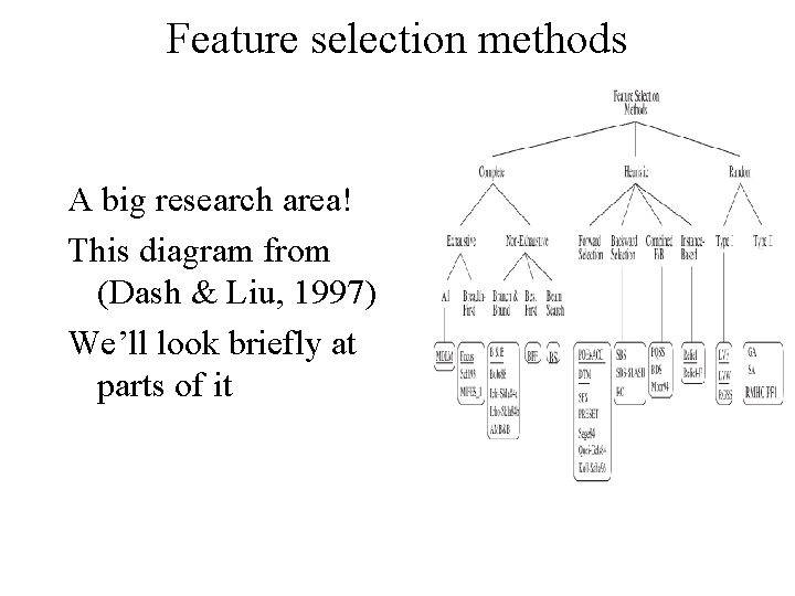
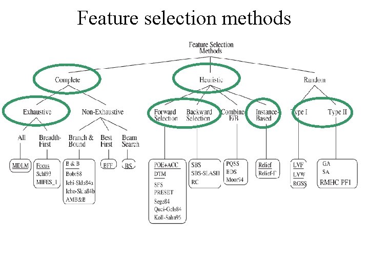
Feature selection methods A big research area! This diagram from (Dash & Liu, 1997) We’ll look briefly at parts of it

Feature selection methods

Feature selection methods

Correlation-based feature ranking This is what you will use in CW 2. It is indeed used often, by practitioners (who perhaps don’t understand the issues involved in FS) It is actually fine for certain datasets. It is not even considered in Dash & Liu’s survey.

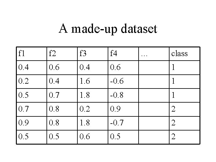
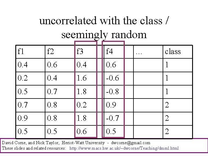
A made-up dataset f 1 f 2 f 3 f 4 … class 0. 4 0. 6 1 0. 2 0. 4 1. 6 -0. 6 1 0. 5 0. 7 1. 8 -0. 8 1 0. 7 0. 8 0. 2 0. 9 0. 8 1. 8 -0. 7 2 0. 5 0. 6 0. 5 2

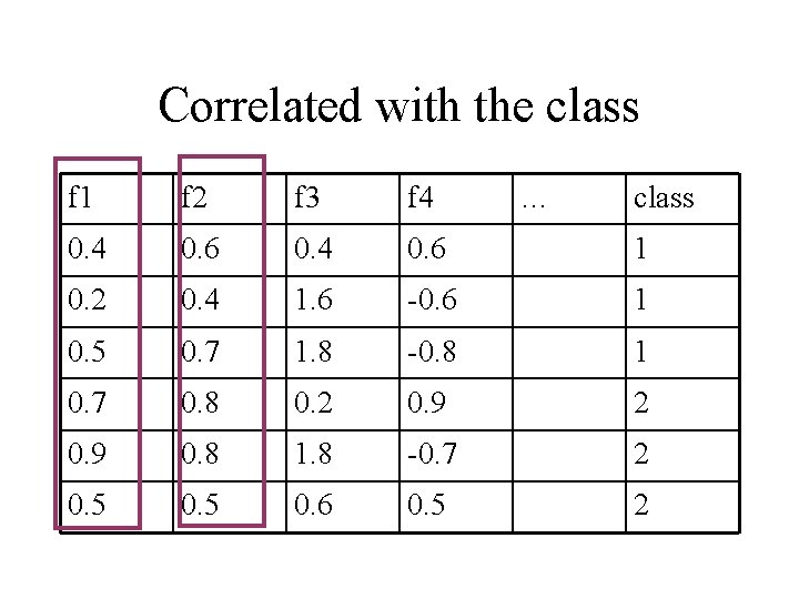
Correlated with the class f 1 f 2 f 3 f 4 … class 0. 4 0. 6 1 0. 2 0. 4 1. 6 -0. 6 1 0. 5 0. 7 1. 8 -0. 8 1 0. 7 0. 8 0. 2 0. 9 0. 8 1. 8 -0. 7 2 0. 5 0. 6 0. 5 2

uncorrelated with the class / seemingly random f 1 f 2 f 3 f 4 … class 0. 4 0. 6 1 0. 2 0. 4 1. 6 -0. 6 1 0. 5 0. 7 1. 8 -0. 8 1 0. 7 0. 8 0. 2 0. 9 0. 8 1. 8 -0. 7 2 0. 5 0. 6 0. 5 2 David Corne, and Nick Taylor, Heriot-Watt University - dwcorne@gmail. com These slides and related resources: http: //www. macs. hw. ac. uk/~dwcorne/Teaching/dmml. html

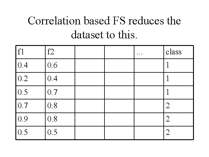
Correlation based FS reduces the dataset to this. f 1 f 2 … class 0. 4 0. 6 1 0. 2 0. 4 1 0. 5 0. 7 1 0. 7 0. 8 2 0. 9 0. 8 2 0. 5 2

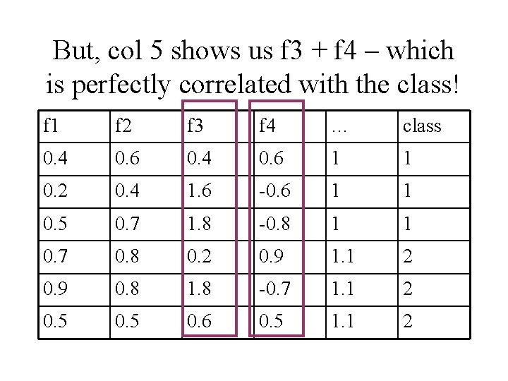
But, col 5 shows us f 3 + f 4 – which is perfectly correlated with the class! f 1 f 2 f 3 f 4 … class 0. 4 0. 6 1 1 0. 2 0. 4 1. 6 -0. 6 1 1 0. 5 0. 7 1. 8 -0. 8 1 1 0. 7 0. 8 0. 2 0. 9 1. 1 2 0. 9 0. 8 1. 8 -0. 7 1. 1 2 0. 5 0. 6 0. 5 1. 1 2

Good FS Methods therefore: • Need to consider how well features work together • As we have noted before, if you take 100 features that are each well correlated with the class, they may simply be correlated strongly with each other, so provide no more information than just one of them

`Complete’ methods Original dataset has N features You want to use a subset of k features A complete FS method means: try every subset of k features, and choose the best! the number of subsets is N! / k!(N−k)! what is this when N is 100 and k is 5?

`Complete’ methods Original dataset has N features You want to use a subset of k features A complete FS method means: try every subset of k features, and choose the best! the number of subsets is N! / k!(N−k)! what is this when N is 100 and k is 5? 75, 287, 520 -- almost nothing

`Complete’ methods Original dataset has N features You want to use a subset of k features A complete FS method means: try every subset of k features, and choose the best! the number of subsets is N! / k!(N−k)! what is this when N is 10, 000 and k is 100?

`Complete’ methods Original dataset has N features You want to use a subset of k features A complete FS method means: try every subset of k features, and choose the best! the number of subsets is N! / k!(N−k)! what is this when N is 10, 000 and k is 100? 5, 000, 000, 000, Continued 1 …. .

000, 000, 000, 000, 000, 000, 000, 000, 000, 000, 000, 000, 000, 000, 000, 000, 000, 000, 000, 000, 000, 000, 000, 000, 000, Continued 2 …. .

000, 000, 000, 000, 000, 000, 000, 000, 000, 000, 000, 000, 000, 000, 000, 000, 000, 000, 000, 000, 000, 000, 000, 000, 000, Continued 3 …. .

000, 000, 000, 000, 000, 000, 000, 000, 000, 000, 000, 000, 000, 000, 000, 000, 000, 000, 000, 000, 000, 000, 000, 000, 000, Continued 4 …. .

… continued for another 114 slides. Actually it is around 5 × 1035, 101 (there around 1080 atoms in the universe)

Can you see a problem with complete methods?

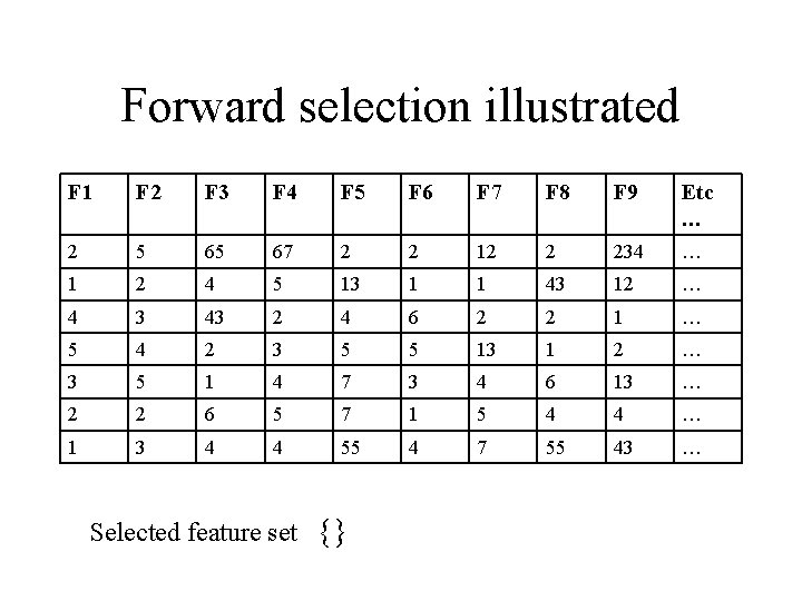
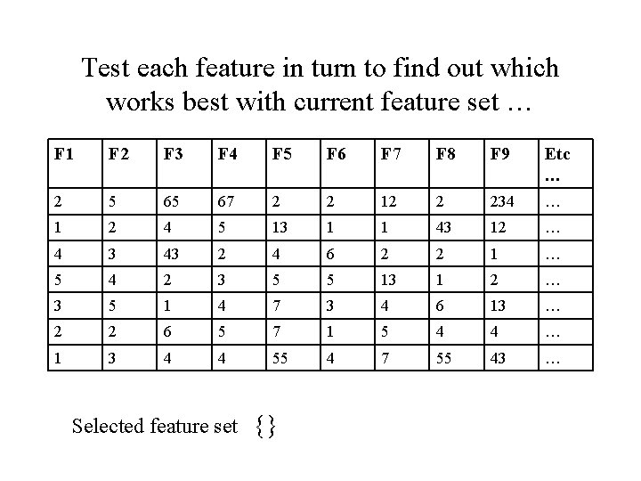
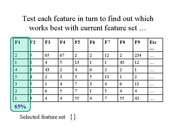
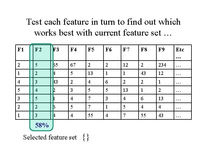
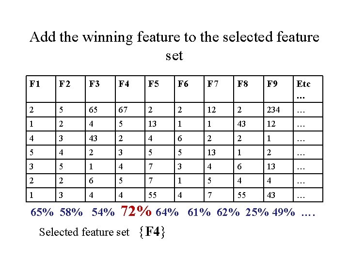
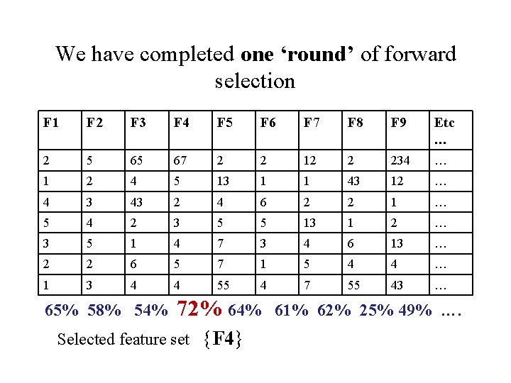
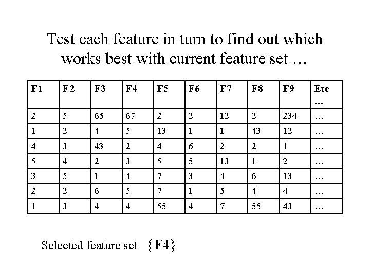
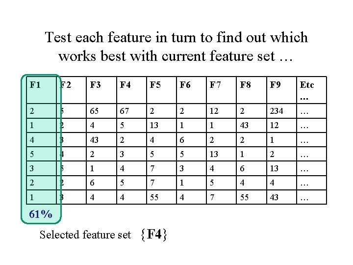
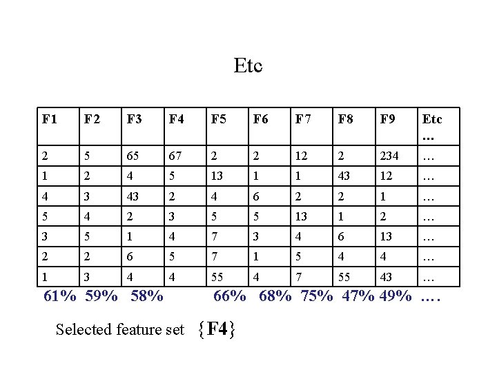
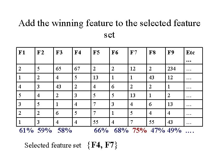
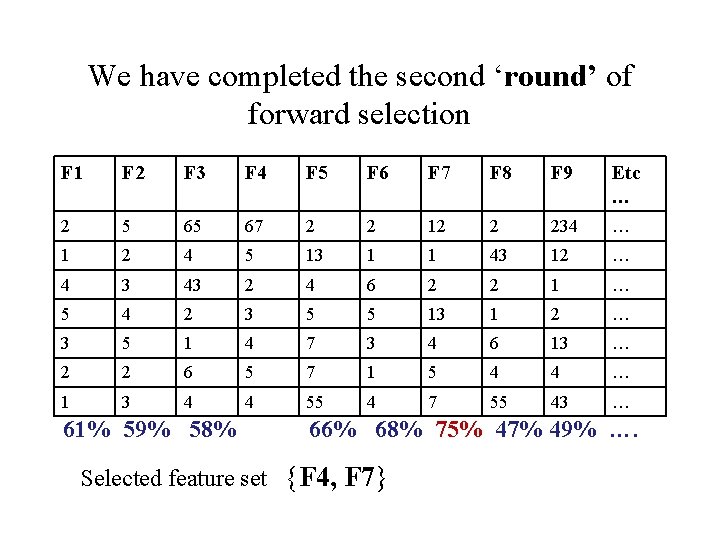
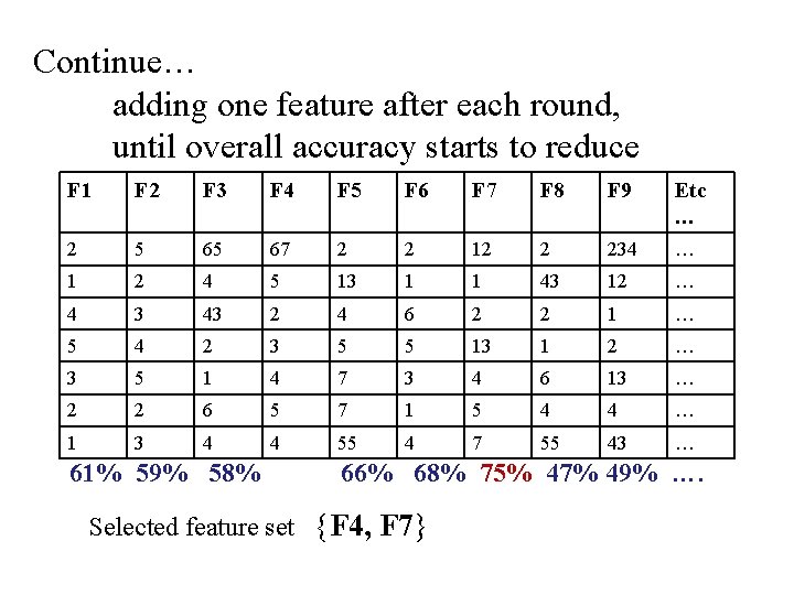
`Forward’ methods These methods `grow’ a set S of features – • S starts empty • Find the best feature to add (by checking which one gives best performance on a test set when combined with S). • If overall performance has improved, return to step 2; else stop

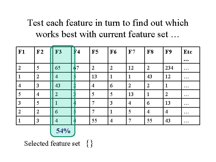
Forward selection illustrated F 1 F 2 F 3 F 4 F 5 F 6 F 7 F 8 F 9 Etc … 2 5 65 67 2 2 12 2 234 … 1 2 4 5 13 1 1 43 12 … 4 3 43 2 4 6 2 2 1 … 5 4 2 3 5 5 13 1 2 … 3 5 1 4 7 3 4 6 13 … 2 2 6 5 7 1 5 4 4 … 1 3 4 4 55 4 7 55 43 … Selected feature set {}

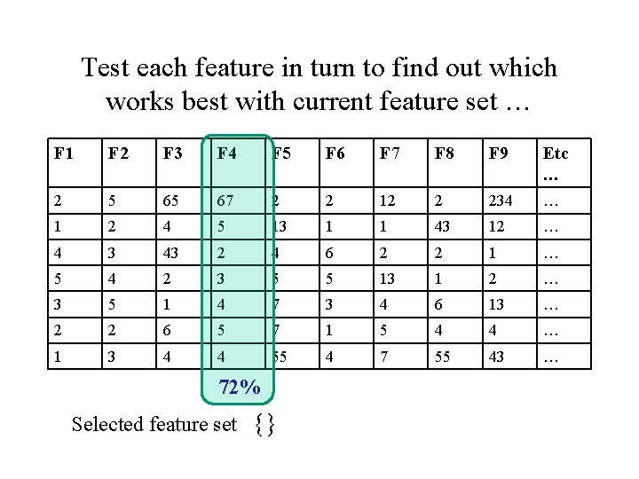
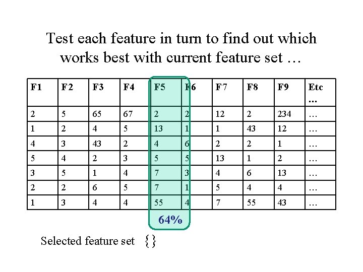
Test each feature in turn to find out which works best with current feature set … F 1 F 2 F 3 F 4 F 5 F 6 F 7 F 8 F 9 Etc … 2 5 65 67 2 2 12 2 234 … 1 2 4 5 13 1 1 43 12 … 4 3 43 2 4 6 2 2 1 … 5 4 2 3 5 5 13 1 2 … 3 5 1 4 7 3 4 6 13 … 2 2 6 5 7 1 5 4 4 … 1 3 4 4 55 4 7 55 43 … Selected feature set {}

Test each feature in turn to find out which works best with current feature set … F 1 F 2 F 3 F 4 F 5 F 6 F 7 F 8 F 9 Etc … 2 5 65 67 2 2 12 2 234 … 1 2 4 5 13 1 1 43 12 … 4 3 43 2 4 6 2 2 1 … 5 4 2 3 5 5 13 1 2 … 3 5 1 4 7 3 4 6 13 … 2 2 6 5 7 1 5 4 4 … 1 3 4 4 55 4 7 55 43 … 65% Selected feature set {}

Test each feature in turn to find out which works best with current feature set … F 1 F 2 F 3 F 4 F 5 F 6 F 7 F 8 F 9 Etc … 2 5 65 67 2 2 12 2 234 … 1 2 4 5 13 1 1 43 12 … 4 3 43 2 4 6 2 2 1 … 5 4 2 3 5 5 13 1 2 … 3 5 1 4 7 3 4 6 13 … 2 2 6 5 7 1 5 4 4 … 1 3 4 4 55 4 7 55 43 … 58% Selected feature set {}

Test each feature in turn to find out which works best with current feature set … F 1 F 2 F 3 F 4 F 5 F 6 F 7 F 8 F 9 Etc … 2 5 65 67 2 2 12 2 234 … 1 2 4 5 13 1 1 43 12 … 4 3 43 2 4 6 2 2 1 … 5 4 2 3 5 5 13 1 2 … 3 5 1 4 7 3 4 6 13 … 2 2 6 5 7 1 5 4 4 … 1 3 4 4 55 4 7 55 43 … 54% Selected feature set {}

Test each feature in turn to find out which works best with current feature set … F 1 F 2 F 3 F 4 F 5 F 6 F 7 F 8 F 9 Etc … 2 5 65 67 2 2 12 2 234 … 1 2 4 5 13 1 1 43 12 … 4 3 43 2 4 6 2 2 1 … 5 4 2 3 5 5 13 1 2 … 3 5 1 4 7 3 4 6 13 … 2 2 6 5 7 1 5 4 4 … 1 3 4 4 55 4 7 55 43 … 72% Selected feature set {}

Test each feature in turn to find out which works best with current feature set … F 1 F 2 F 3 F 4 F 5 F 6 F 7 F 8 F 9 Etc … 2 5 65 67 2 2 12 2 234 … 1 2 4 5 13 1 1 43 12 … 4 3 43 2 4 6 2 2 1 … 5 4 2 3 5 5 13 1 2 … 3 5 1 4 7 3 4 6 13 … 2 2 6 5 7 1 5 4 4 … 1 3 4 4 55 4 7 55 43 … 64% Selected feature set {}

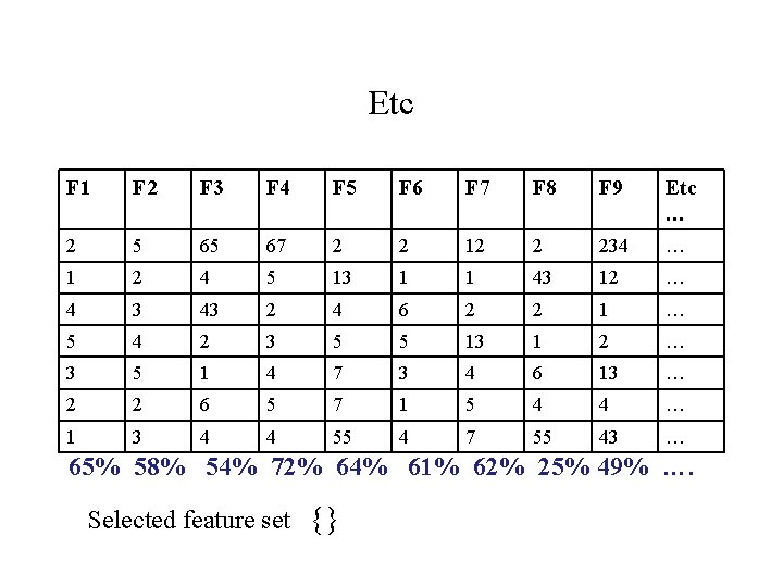
Etc F 1 F 2 F 3 F 4 F 5 F 6 F 7 F 8 F 9 Etc … 2 5 65 67 2 2 12 2 234 … 1 2 4 5 13 1 1 43 12 … 4 3 43 2 4 6 2 2 1 … 5 4 2 3 5 5 13 1 2 … 3 5 1 4 7 3 4 6 13 … 2 2 6 5 7 1 5 4 4 … 1 3 4 4 55 4 7 55 43 … 65% 58% 54% 72% 64% 61% 62% 25% 49% …. Selected feature set {}

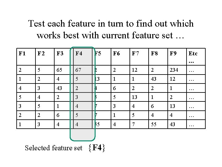
Add the winning feature to the selected feature set F 1 F 2 F 3 F 4 F 5 F 6 F 7 F 8 F 9 Etc … 2 5 65 67 2 2 12 2 234 … 1 2 4 5 13 1 1 43 12 … 4 3 43 2 4 6 2 2 1 … 5 4 2 3 5 5 13 1 2 … 3 5 1 4 7 3 4 6 13 … 2 2 6 5 7 1 5 4 4 … 1 3 4 4 55 4 7 55 43 … 65% 58% 54% 72% 64% Selected feature set {F 4} 61% 62% 25% 49% ….

We have completed one ‘round’ of forward selection F 1 F 2 F 3 F 4 F 5 F 6 F 7 F 8 F 9 Etc … 2 5 65 67 2 2 12 2 234 … 1 2 4 5 13 1 1 43 12 … 4 3 43 2 4 6 2 2 1 … 5 4 2 3 5 5 13 1 2 … 3 5 1 4 7 3 4 6 13 … 2 2 6 5 7 1 5 4 4 … 1 3 4 4 55 4 7 55 43 … 65% 58% 54% 72% 64% Selected feature set {F 4} 61% 62% 25% 49% ….

Test each feature in turn to find out which works best with current feature set … F 1 F 2 F 3 F 4 F 5 F 6 F 7 F 8 F 9 Etc … 2 5 65 67 2 2 12 2 234 … 1 2 4 5 13 1 1 43 12 … 4 3 43 2 4 6 2 2 1 … 5 4 2 3 5 5 13 1 2 … 3 5 1 4 7 3 4 6 13 … 2 2 6 5 7 1 5 4 4 … 1 3 4 4 55 4 7 55 43 … Selected feature set {F 4}

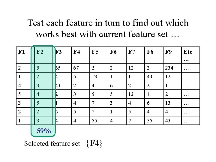
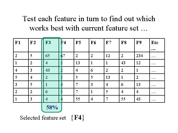
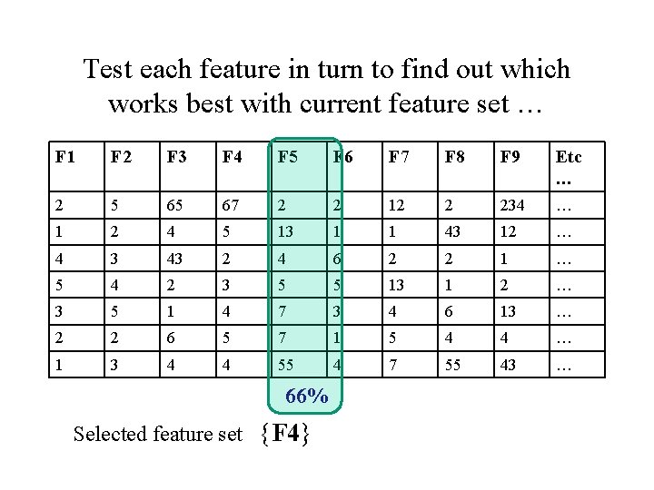
Test each feature in turn to find out which works best with current feature set … F 1 F 2 F 3 F 4 F 5 F 6 F 7 F 8 F 9 Etc … 2 5 65 67 2 2 12 2 234 … 1 2 4 5 13 1 1 43 12 … 4 3 43 2 4 6 2 2 1 … 5 4 2 3 5 5 13 1 2 … 3 5 1 4 7 3 4 6 13 … 2 2 6 5 7 1 5 4 4 … 1 3 4 4 55 4 7 55 43 … 61% Selected feature set {F 4}

Test each feature in turn to find out which works best with current feature set … F 1 F 2 F 3 F 4 F 5 F 6 F 7 F 8 F 9 Etc … 2 5 65 67 2 2 12 2 234 … 1 2 4 5 13 1 1 43 12 … 4 3 43 2 4 6 2 2 1 … 5 4 2 3 5 5 13 1 2 … 3 5 1 4 7 3 4 6 13 … 2 2 6 5 7 1 5 4 4 … 1 3 4 4 55 4 7 55 43 … 59% Selected feature set {F 4}

Test each feature in turn to find out which works best with current feature set … F 1 F 2 F 3 F 4 F 5 F 6 F 7 F 8 F 9 Etc … 2 5 65 67 2 2 12 2 234 … 1 2 4 5 13 1 1 43 12 … 4 3 43 2 4 6 2 2 1 … 5 4 2 3 5 5 13 1 2 … 3 5 1 4 7 3 4 6 13 … 2 2 6 5 7 1 5 4 4 … 1 3 4 4 55 4 7 55 43 … 58% Selected feature set {F 4}

Test each feature in turn to find out which works best with current feature set … F 1 F 2 F 3 F 4 F 5 F 6 F 7 F 8 F 9 Etc … 2 5 65 67 2 2 12 2 234 … 1 2 4 5 13 1 1 43 12 … 4 3 43 2 4 6 2 2 1 … 5 4 2 3 5 5 13 1 2 … 3 5 1 4 7 3 4 6 13 … 2 2 6 5 7 1 5 4 4 … 1 3 4 4 55 4 7 55 43 … Selected feature set {F 4}

Test each feature in turn to find out which works best with current feature set … F 1 F 2 F 3 F 4 F 5 F 6 F 7 F 8 F 9 Etc … 2 5 65 67 2 2 12 2 234 … 1 2 4 5 13 1 1 43 12 … 4 3 43 2 4 6 2 2 1 … 5 4 2 3 5 5 13 1 2 … 3 5 1 4 7 3 4 6 13 … 2 2 6 5 7 1 5 4 4 … 1 3 4 4 55 4 7 55 43 … 66% Selected feature set {F 4}

Etc F 1 F 2 F 3 F 4 F 5 F 6 F 7 F 8 F 9 Etc … 2 5 65 67 2 2 12 2 234 … 1 2 4 5 13 1 1 43 12 … 4 3 43 2 4 6 2 2 1 … 5 4 2 3 5 5 13 1 2 … 3 5 1 4 7 3 4 6 13 … 2 2 6 5 7 1 5 4 4 … 1 3 4 4 55 4 7 55 43 … 61% 59% 58% 66% 68% 75% 47% 49% …. Selected feature set {F 4}

Add the winning feature to the selected feature set F 1 F 2 F 3 F 4 F 5 F 6 F 7 F 8 F 9 Etc … 2 5 65 67 2 2 12 2 234 … 1 2 4 5 13 1 1 43 12 … 4 3 43 2 4 6 2 2 1 … 5 4 2 3 5 5 13 1 2 … 3 5 1 4 7 3 4 6 13 … 2 2 6 5 7 1 5 4 4 … 1 3 4 4 55 4 7 55 43 … 61% 59% 58% 66% 68% 75% 47% 49% …. Selected feature set {F 4, F 7}

We have completed the second ‘round’ of forward selection F 1 F 2 F 3 F 4 F 5 F 6 F 7 F 8 F 9 Etc … 2 5 65 67 2 2 12 2 234 … 1 2 4 5 13 1 1 43 12 … 4 3 43 2 4 6 2 2 1 … 5 4 2 3 5 5 13 1 2 … 3 5 1 4 7 3 4 6 13 … 2 2 6 5 7 1 5 4 4 … 1 3 4 4 55 4 7 55 43 … 61% 59% 58% 66% 68% 75% 47% 49% …. Selected feature set {F 4, F 7}

Continue… adding one feature after each round, until overall accuracy starts to reduce F 1 F 2 F 3 F 4 F 5 F 6 F 7 F 8 F 9 Etc … 2 5 65 67 2 2 12 2 234 … 1 2 4 5 13 1 1 43 12 … 4 3 43 2 4 6 2 2 1 … 5 4 2 3 5 5 13 1 2 … 3 5 1 4 7 3 4 6 13 … 2 2 6 5 7 1 5 4 4 … 1 3 4 4 55 4 7 55 43 … 61% 59% 58% 66% 68% 75% 47% 49% …. Selected feature set {F 4, F 7}

`Backward’ methods These methods remove features one by one. • S starts with the full feature set • Find the best feature to remove (by checking which removal from S gives best performance on a test set). • If overall performance has improved, return to step 2; else stop

• When might you choose forward instead of backward?

Random(ised) methods aka Stochastic methods Suppose you have 1, 000 features. There are 21000 possible subsets of features. One way to try to find a good subset is to run a stochastic search algorithm E. g. Hillclimbing, simulated annealing, genetic algorithm, particle swarm optimisation, …

Example to give flavour of heuristic methods Forward selection works by, in each round, adding ONE feature to the growing set, having tried every feature in turn. If there are 50, 000 features, how many steps in each round?

Example to give flavour of heuristic methods Forward selection works by, in each round, adding ONE feature to the growing set, having tried every feature in turn. If there are 50, 000 features, how many steps in each round? What if, in each round, you wanted to find the best pair of features to add, how many steps would there be per round?

Example to give flavour of heuristic methods Forward selection works by, in each round, adding ONE feature to the growing set, having tried every feature in turn. If there are 50, 000 features, how many steps in each round? What if, in each round, you wanted to find the best pair of features to add, how many steps would there be per round? So, what could you do instead, to make this a workable method?

Why randomised/search methods are good for FS Usually you have a large number of features (e. g. 1, 000) You can give each feature a score (e. g. correlation with target, Relief weight (see end slides), etc …), and choose the best-scoring features. This is very fast. However this does not evaluate how well features work with other features. You could give combinations of features a score, but there are too many combinations of multiple features. Search algorithms are the only suitable approach that get to grips with evaluating combinations of features.

If time: the classic example of an instance-based heuristic method

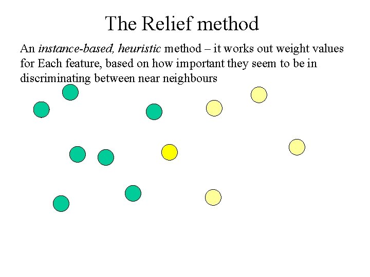
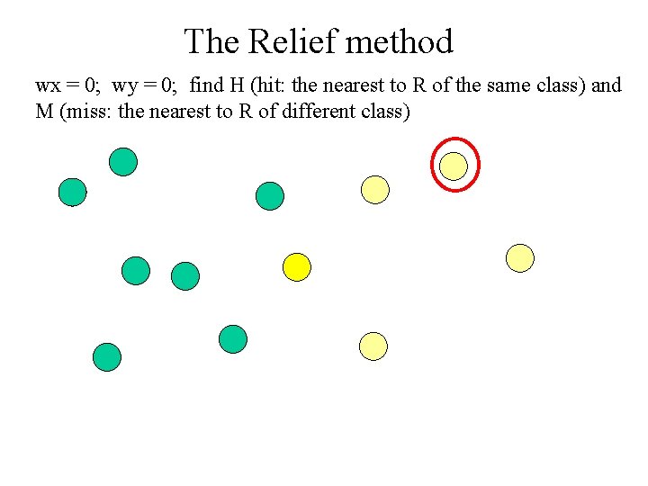
The Relief method An instance-based, heuristic method – it works out weight values for Each feature, based on how important they seem to be in discriminating between near neighbours

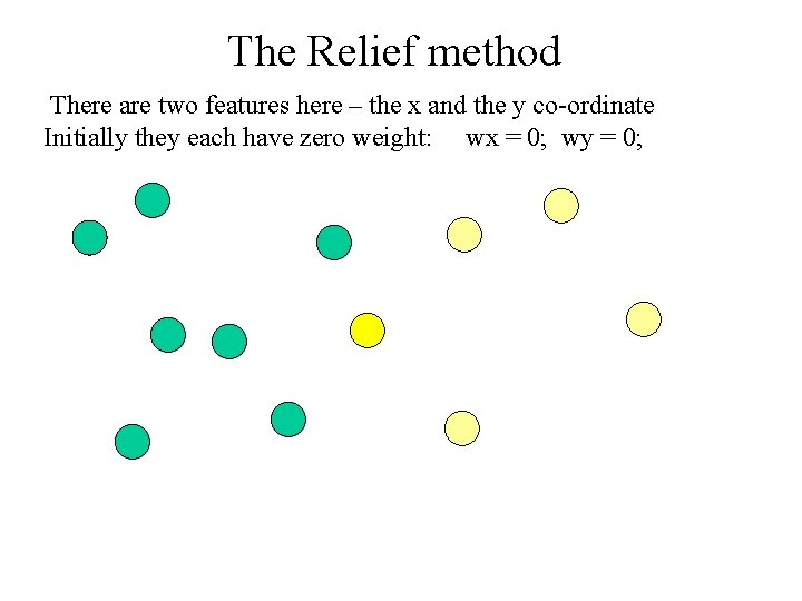
The Relief method There are two features here – the x and the y co-ordinate Initially they each have zero weight: wx = 0; wy = 0;

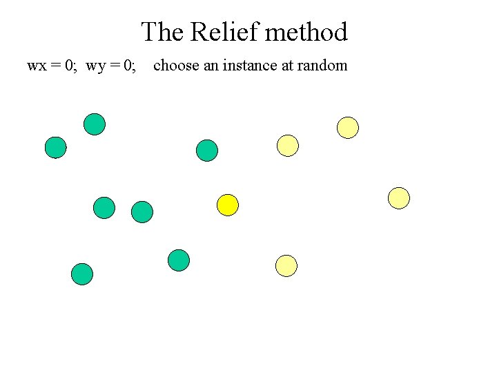
The Relief method wx = 0; wy = 0; choose an instance at random

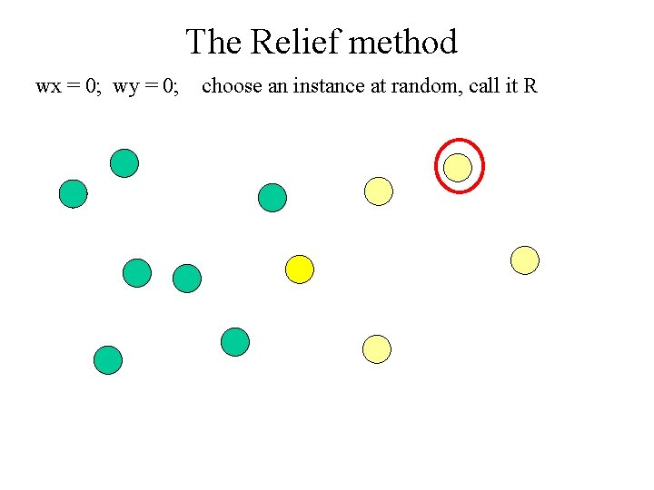
The Relief method wx = 0; wy = 0; choose an instance at random, call it R

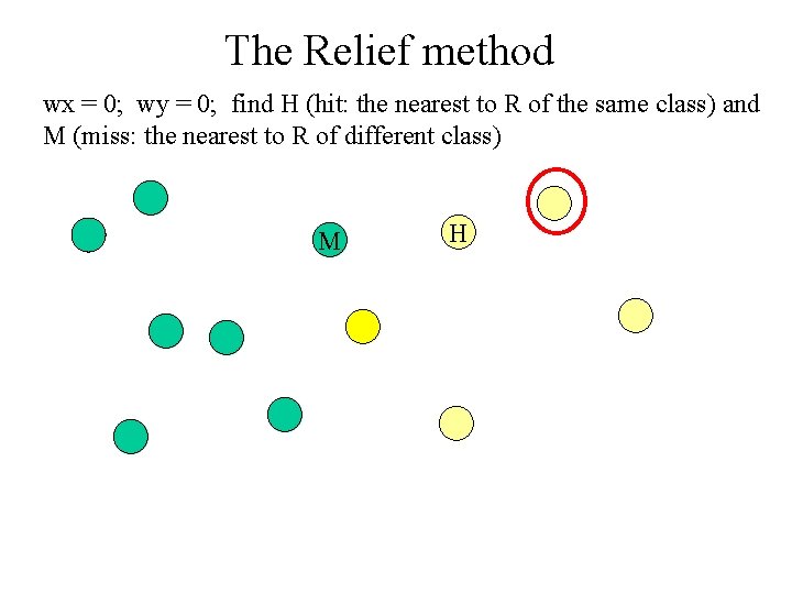
The Relief method wx = 0; wy = 0; find H (hit: the nearest to R of the same class) and M (miss: the nearest to R of different class)

The Relief method wx = 0; wy = 0; find H (hit: the nearest to R of the same class) and M (miss: the nearest to R of different class) M H

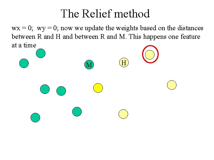
The Relief method wx = 0; wy = 0; now we update the weights based on the distances between R and H and between R and M. This happens one feature at a time M H

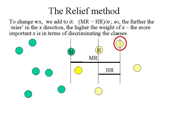
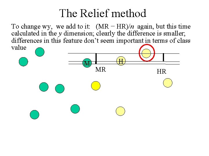
The Relief method To change wx, we add to it: (MR − HR)/n ; so, the further the `miss’ in the x direction, the higher the weight of x – the more important x is in terms of discriminating the classes M H MR HR

The Relief method To change wy, we add to it: (MR − HR)/n again, but this time calculated in the y dimension; clearly the difference is smaller; differences in this feature don’t seem important in terms of class value M H MR HR

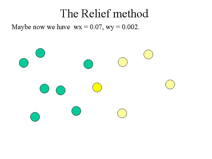
The Relief method Maybe now we have wx = 0. 07, wy = 0. 002.

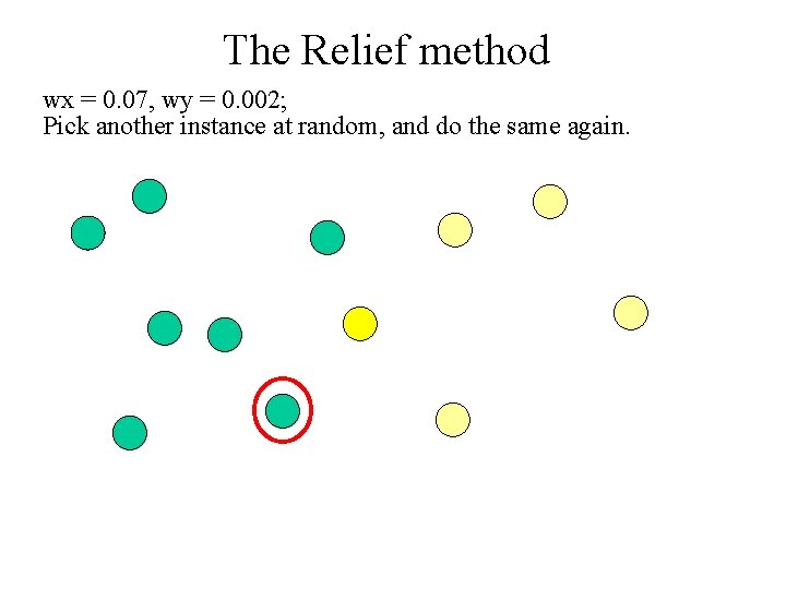
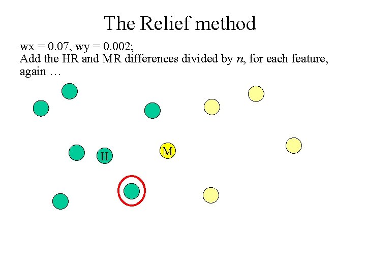
The Relief method wx = 0. 07, wy = 0. 002; Pick another instance at random, and do the same again.

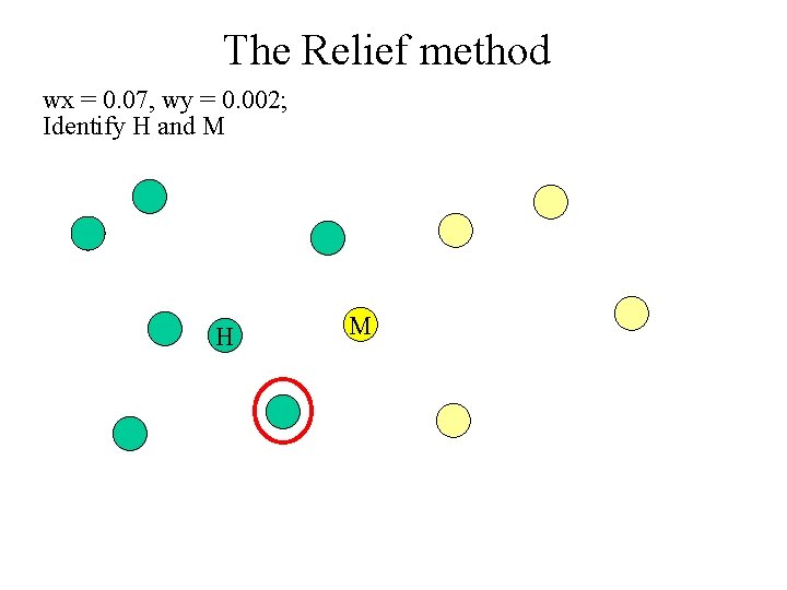
The Relief method wx = 0. 07, wy = 0. 002; Identify H and M H M

The Relief method wx = 0. 07, wy = 0. 002; Add the HR and MR differences divided by n, for each feature, again … H M

The Relief method In the end, we have a weight value for each feature. The higher the value, the more relevant the feature. We can use these weights for feature selection, simply by choosing the features with the S highest weights (if we want to use S features) NOTE -It is important to use Relief F only on min-max normalised data in [0, 1]. However it is fine if category attibutes are involved, in which case use Hamming distance for those attributes, -Why divide by n? Then, the weight values can be interpreted as a difference in probabilities.

The Relief method, plucked directly from the original paper (Kira and Rendell 1992)